Day 9: Regularization — Ridge, Lasso, ElasticNet

Day 2 introduced overfitting. Day 3 framed it as a variance problem. Today we meet the cleanest, most asked-about tool to fix it in linear models: Regularisation. If an interviewer asks "how do you stop a model from overfitting?", half of the right answer lives in this post.

This blog post is a daily learning summary of my ML self-study.

Heads-up (Cross-validation in 30 seconds): A few code examples below use RidgeCV, which automatically tries several alpha values and picks the best one. The "CV" part means it splits our training data into chunks, trains on some chunks, tests on the others, repeats, and averages the result. We will fully cover cross-validation on Day 10 Cross-Validation & Hyperparameter Tuning.

Terms Used Today

Regularisation: Adding a penalty on coefficient size to the loss, so the model cannot grow wild coefficients.

L2 penalty (Ridge): Penalises the sum of squared coefficients. Shrinks all coefficients but keeps them.

L1 penalty (Lasso): Penalises the sum of absolute coefficients. Can drive some coefficients to exactly zero (automatic feature selection).

ElasticNet: Combines L1 and L2 penalties.

λ (lambda): The strength of the penalty in our formulas. 0 means no penalty, large means harsh. (In sklearn code this knob is exposed as the alpha parameter; different naming, same idea.)

α (alpha) in ElasticNet: A separate knob that controls the mix between L1 and L2 penalties. In sklearn, this is exposed as l1_ratio.

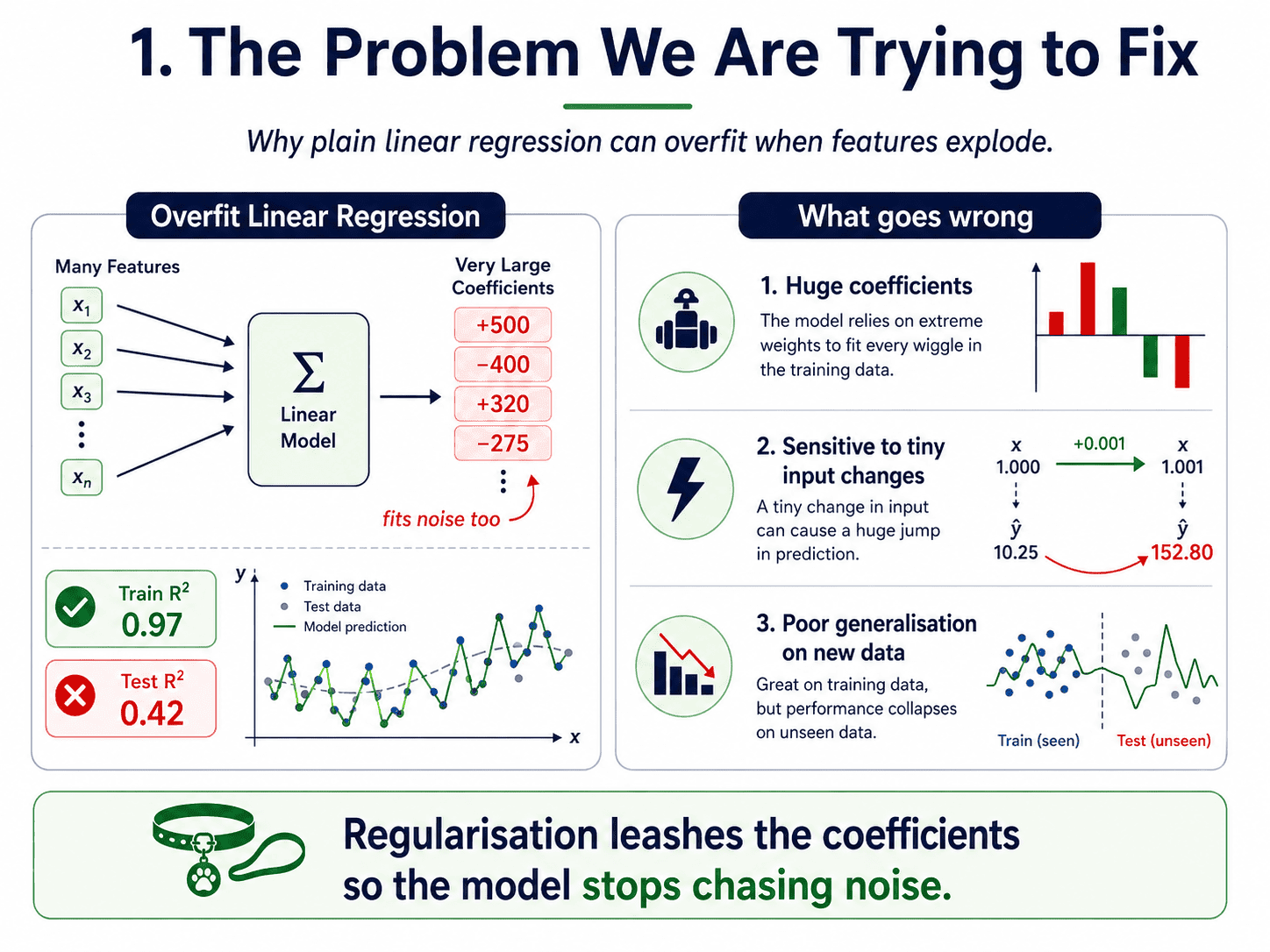
1. The Problem We Are Trying to Fix:

A Linear Regression with too many features (relative to the data) can fit the training data beautifully, including its noise. The coefficients grow huge to chase every wiggle. Then new data arrives, the model overreacts, and the test score collapses.

The symptoms are familiar.

Train R² = 0.97, Test R² = 0.42 (classic overfitting).
Coefficients are wildly large: some +500, some −400.
Tiny changes in inputs cause wild changes in outputs.

We need a way to leash the model. That is what Regularisation does.

2. The Big Idea:

We modify the loss function so the model is penalised for using large coefficients.

Why? Because large coefficients make the model highly sensitive to small changes in the input, and that sensitivity is exactly what causes overfitting.

Loss = Data Error + Regularisation Penalty

So we are no longer just asking "fit the data well."

We are also asking "stay simple while doing it."

Two competing pressures.

Fit the data well.
Keep coefficients small.

And here is the connection back to Day 3: Bias-Variance Tradeoff — Why Models Fail. By shrinking coefficients, we reduce how sensitive the model is to small changes in data, which is exactly what variance is.

So regularisation is, fundamentally, a variance-control tool.

The balance between fitting and staying simple is controlled by one knob, called λ (lambda) in textbooks. (In sklearn code, this knob is named alpha, but mathematically it is λ. We will stick with λ in the formulas to keep things clean.)

λ = 0 → no penalty. Behaves like regular Linear Regression.
λ very large → coefficients squashed toward zero. Underfitting.
λ just right → the sweet spot.

A small but important point. As we increase λ, variance goes down, but bias goes up. Regularisation is a tradeoff, not a free win. It is the bias-variance seesaw with a new dial.

A Quick Concrete Picture:

Before the math, let us see what regularisation does to coefficients in practice. Imagine a Linear Regression on 1,000 features that overfit hard and produced coefficients like:

Before: [+420, −380, +295, ..., +310, −275]

After applying Ridge regularisation, those same coefficients might look like:

After Ridge: [+3.2, −2.8, +1.9, ..., +2.4, −1.7]

Same model, but less sensitive to noise because the coefficients are leashed. Lasso would go further and zero out the useless ones entirely:

After Lasso: [+3.1, 0, +1.8, ..., 0, 0]

That is the whole story. Now to the math.

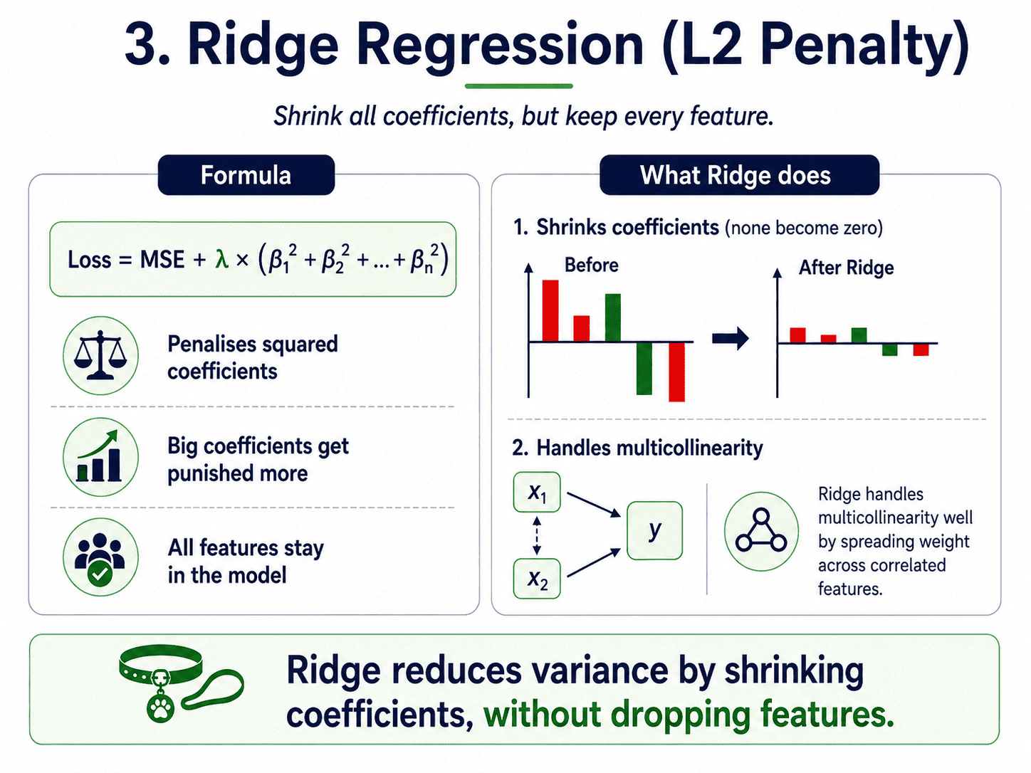
3. Ridge Regression (L2 Penalty):

Penalise the sum of squared coefficients.

Loss = MSE + λ × (β₁² + β₂² + ... + βₙ²)

The effect is to shrink all coefficients toward zero, but rarely all the way to zero. Big coefficients get punished more (because of squaring), so wild values get flattened first.

Reduces variance.
All features stay in the model, just with smaller coefficients.
Best when many features each contribute a small amount.
Especially useful when features are highly correlated (multicollinearity): Ridge spreads the weight across them instead of picking one arbitrarily.

from sklearn.linear_model import Ridge
model = Ridge(alpha=1.0)
model.fit(X_train, y_train)

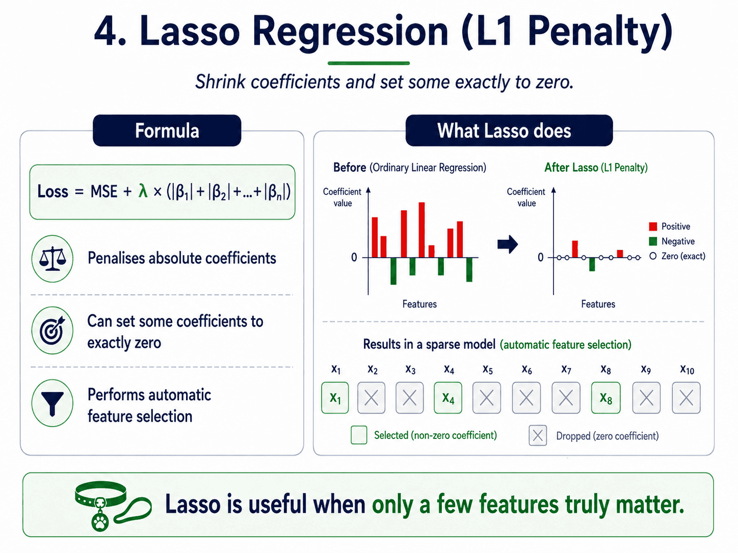
4. Lasso Regression (L1 Penalty):

Penalise the sum of absolute coefficients.

Loss = MSE + λ × (|β₁| + |β₂| + ... + |βₙ|)

The effect is to shrink coefficients toward zero and to set some of them exactly to zero. That is the magic of Lasso: it performs automatic feature selection.

Coefficients of unimportant features become 0, and those features effectively drop out of the model.
Best when we believe only a few features actually matter (though it can be unstable when features are highly correlated, which is exactly where ElasticNet steps in).
Gives us a sparser, more interpretable model.

from sklearn.linear_model import Lasso
model = Lasso(alpha=0.1)
model.fit(X_train, y_train)
print((model.coef_ != 0).sum(), "features kept")

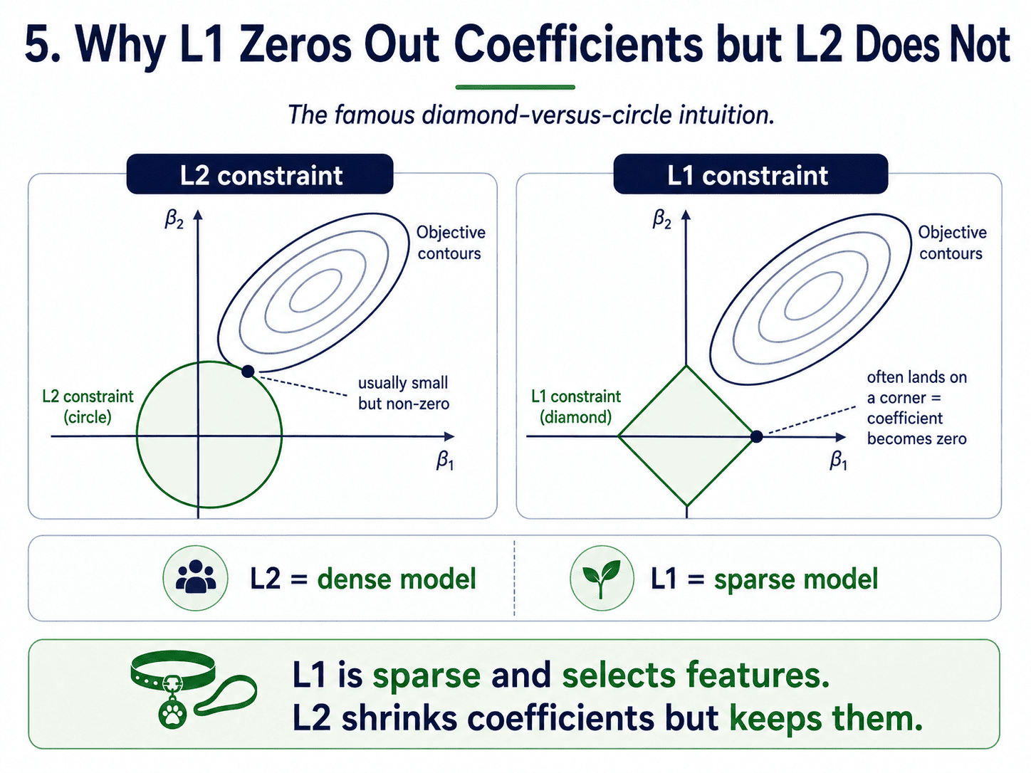
5. Why L1 Zeros Out Coefficients but L2 Does Not (The Intuition):

If we have seen the famous "diamond vs circle" picture in textbooks, here is what it is saying.

The L2 (squared) penalty has round contours. The model meets the constraint somewhere on the curve, usually with small but non-zero coefficients.
The L1 (absolute) penalty has pointy diamond-shaped contours. The model is far more likely to land at a corner of the diamond, and corners sit on the axes, where coefficients are exactly zero.

We do not need the picture. We just need to remember: L1 is sparse (drops features), L2 is small but everyone stays.

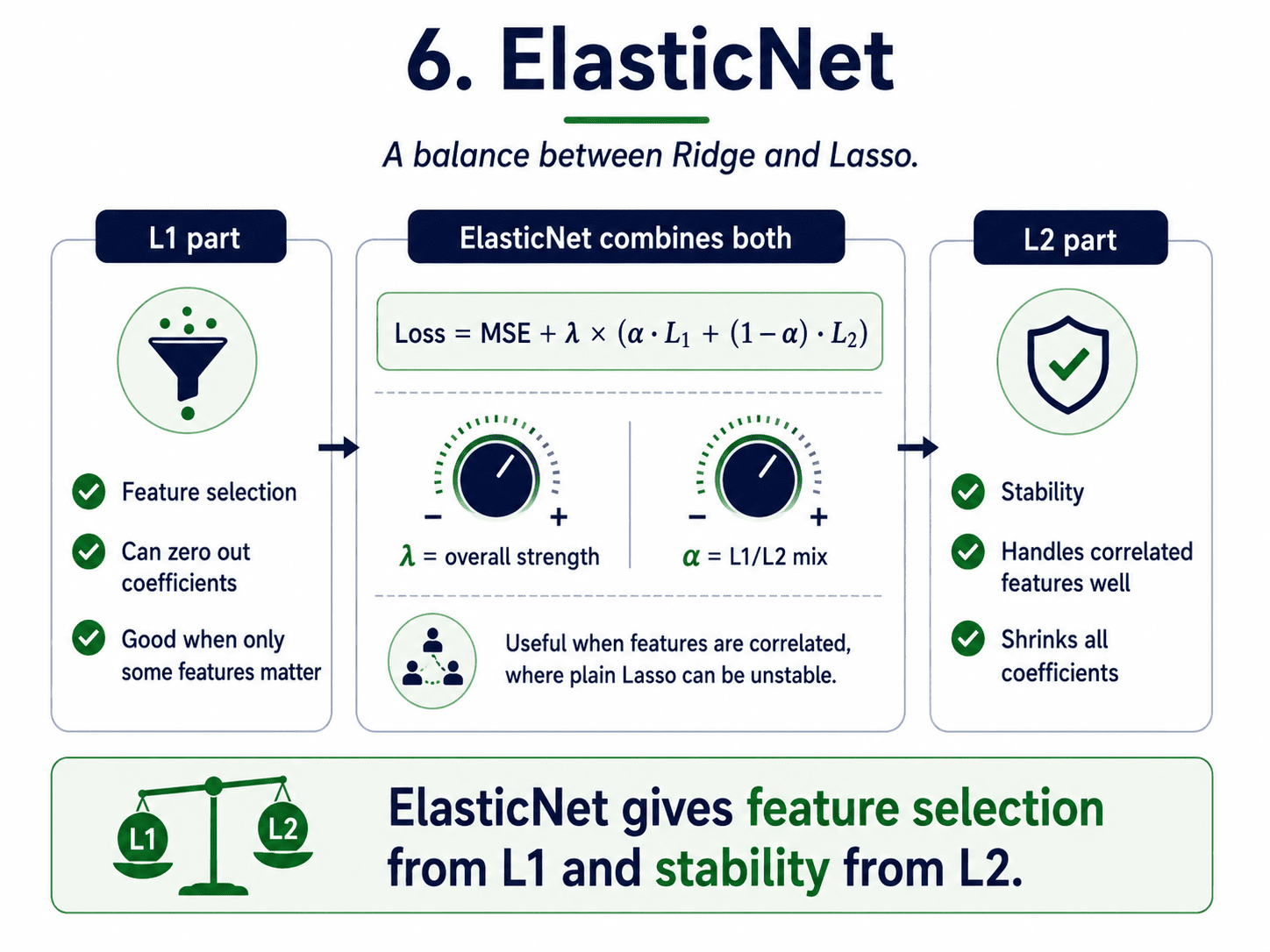
6. ElasticNet:

Use both penalties together with a mixing ratio.

Loss = MSE + λ × (α · L1 + (1 − α) · L2)

This is where the two Greek letters earn their separate roles. α controls the mix between L1 and L2. λ controls the overall strength. Two different knobs, often confused.

We get feature selection from the L1 part.
We get stability from the L2 part.
Especially helpful when features are highly correlated. Lasso alone tends to pick one and ignore the rest, which can be unstable across different samples. ElasticNet is more graceful.

from sklearn.linear_model import ElasticNet
model = ElasticNet(alpha=0.5, l1_ratio=0.5)
model.fit(X_train, y_train)

7. Picking the Right Penalty Strength (λ):

We do not guess λ. We let cross-validation pick it. (In the sklearn code below, λ is the alphas parameter; same idea, different name.)

from sklearn.linear_model import RidgeCV
model = RidgeCV(alphas=[0.001, 0.01, 0.1, 1, 10, 100])
model.fit(X_train, y_train)
print(model.alpha_)   # the λ value chosen by CV

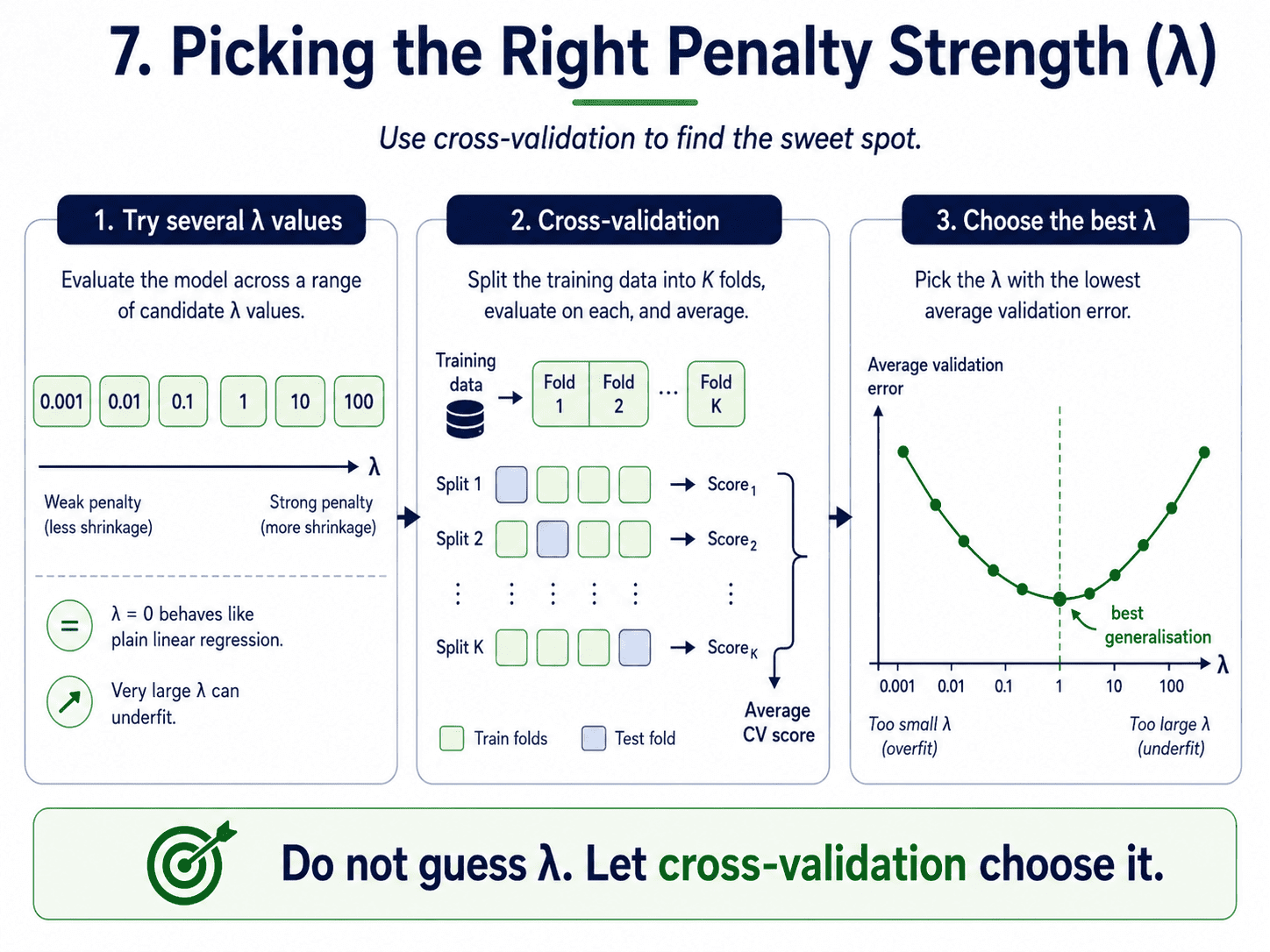
Day 10: Cross-Validation & Hyperparameter Tuning will make cross-validation rigorous. For today, this is the practical pattern.

A Visual Mental Model:

Think of λ as a single dial with three settings.

Too low → the model chases noise (overfit).
Too high → the model becomes too simple (underfit).
Just right → the sweet spot for generalisation.

Cross-validation is how we find "just right."

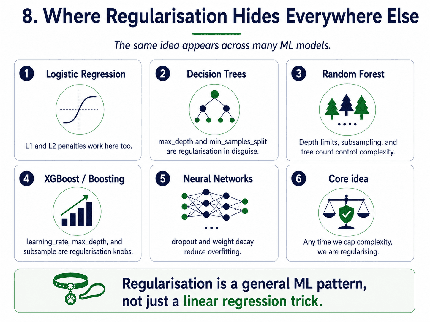
8. Where Regularisation Hides Everywhere Else:

Regularisation is not a specific algorithm. It is a pattern that shows up everywhere in ML. The same "penalise complexity" idea appears across many models, just under different names.

Logistic Regression has the same Ridge/Lasso variants (sklearn calls it penalty='l1' or 'l2').
Decision Trees: max_depth, min_samples_split are regularisation in disguise.
Random Forest and XGBoost: n_estimators, max_depth, learning_rate, subsample.
Neural Networks: dropout, weight decay.

Anytime we put a complexity cap on a model, we are regularising.

A small thought to sit with. Suppose our Linear Regression has 1,000 features but we suspect only ~30 of them are useful. Which regulariser would we reach for? Lasso. It will push the useless coefficients to exactly zero, effectively giving us a 30-feature model. Ridge would keep all 1,000 alive, just smaller. Harder to interpret and not really doing feature selection.

9. A Few Common Confusions Cleared:

Why do I always have to scale features for regularised models? Because regularisation compares coefficient sizes. If features are on different scales, the comparison becomes unfair. Always use StandardScaler before regularising.
Should I regularise the intercept? No, only the slope coefficients. sklearn handles this for us.
Why does Lasso "drop features" while Ridge does not? Because the absolute-value penalty has a non-differentiable corner at zero, and the optimiser is happy to sit exactly on that corner. Squared penalties are smooth everywhere and never quite touch zero.
What if I am not sure between Ridge and Lasso? ElasticNet, then let CV pick the mixing ratio. Or just use Ridge first as a safe default.
Common interview question: "What is the difference between L1 and L2?" L1 = sum of absolute values = sparse / feature selection. L2 = sum of squares = small but dense. Memorise that one line.

10. If This Came In An Interview:

A few questions to be ready for, with one-line answers we should have on the tip of our tongue.

What is regularisation? Adding a penalty on coefficient size to the loss, so the model is discouraged from being overly complex. It is the main way to control variance in linear models.
L1 vs L2? L1 (Lasso) is the sum of absolute coefficients: it can zero out features (automatic feature selection). L2 (Ridge) is the sum of squared coefficients: it shrinks all coefficients but keeps them.
When would you use Lasso over Ridge? When we believe only a few features actually matter. Lasso will drop the rest. Ridge is safer when many features each contribute a little.
What is ElasticNet for? Combines L1 and L2. Especially helpful when features are correlated, since Lasso alone tends to randomly pick one and drop the rest.
What happens as λ increases? Variance goes down, bias goes up. λ = 0 is plain Linear Regression. Very large λ underfits.
Why must features be scaled before regularising? Because the penalty caps every coefficient equally. Features on different scales would get unfair treatment.

11. Summing It Up:

If we remember one thing from today, it is this: regularisation controls model complexity by penalising large coefficients. Ridge shrinks. Lasso selects. ElasticNet balances. λ decides how strict we are. It is the single most common variance-control tool in ML.

Coming Up on Day 10: Cross-Validation & Hyperparameter Tuning

We have leaned on "use cross-validation" three times now. Tomorrow we finally give it the day it deserves, along with the question of how to find the best hyperparameters in general. We will cover K-fold CV, the difference between parameters and hyperparameters, and the contrast between GridSearch and RandomSearch.

That's all for today. Let's meet up again tomorrow with Day 10.

Thanks for reading.

Cheers!