Day 8: Feature Engineering & Preprocessing

There is a saying in ML: "garbage in, garbage out." The fanciest model in the world cannot save us from bad inputs. Today we cover the most underrated, most interview-relevant skill in ML, which is turning raw data into something a model can actually learn from. Senior data scientists say that in real projects, sixty to eighty percent of the time is spent on data work, and only the rest on modelling.

This blog post is a daily learning summary of my ML self-study.

Terms Used Today

Imputation: Filling in missing values (using mean, median, mode, or a constant).

One-hot encoding: Turning a categorical column into many binary columns.

Label encoding: Replacing each category with an integer (creates a fake order).

Target encoding: Replacing each category with the mean target value for that group.

Standardisation (Z-score): Rescale features so mean = 0 and std = 1.

Min-Max scaling: Rescale features to lie in the [0, 1] range.

Pipeline: An sklearn helper that chains preprocessing and the model together, so the same steps run identically on train and test.

Data leakage: When information from test data (or from the future, or from the target) sneaks into training. We will fully cover this on [[Day 22 Data Leakage, ML Workflow & Interview Cheat Sheet|Day 22]].

1. What Raw Data Actually Looks Like:

Real data is messy. Some of the regulars we will meet are:

Missing values (NaN, empty strings, "?", or sentinel values like −99).
Categorical columns (red, blue, green).
Numerical columns on wildly different scales (age in years vs salary in dollars).
Outliers (a $50M house in a suburban dataset).
Dates and times in many different formats.
Strings that should be numbers.
The same category written five different ways (USA, U.S.A, United States, us).

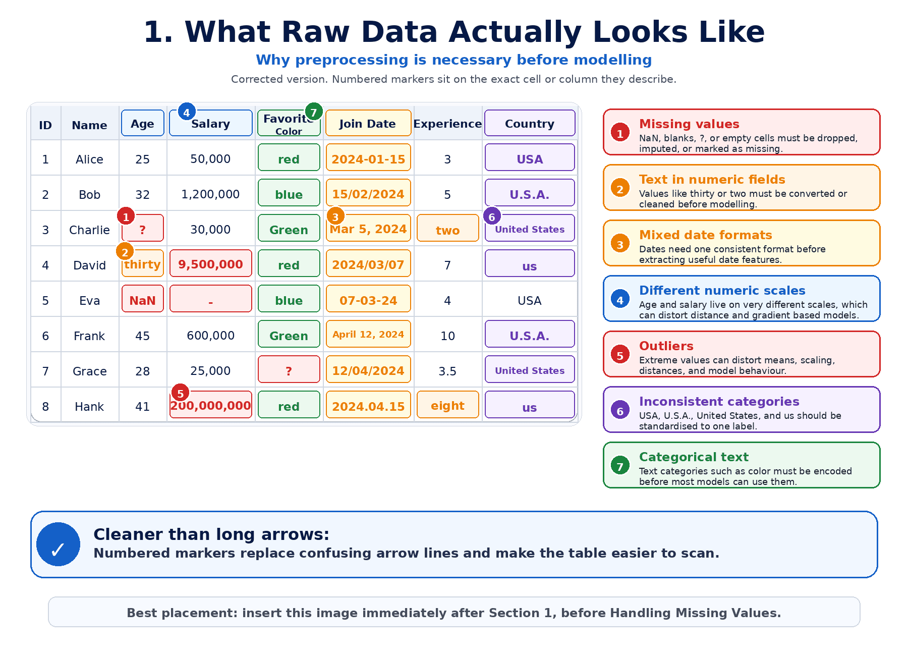
None of this fits into a model directly. We have to clean and transform.

2. Handling Missing Values:

Three strategies, in increasing order of effort.

Drop them. If only a tiny fraction (say 1%) of rows have missing values, we drop them and move on. Quick and harmless on big datasets.

Impute them. Replace missing values with something reasonable.

Mean or Median for numeric columns. Median is more robust to outliers.
Mode for categorical columns.
Forward-fill or Backward-fill for time series.
Constant: fill with 0, "Unknown," or another sentinel.

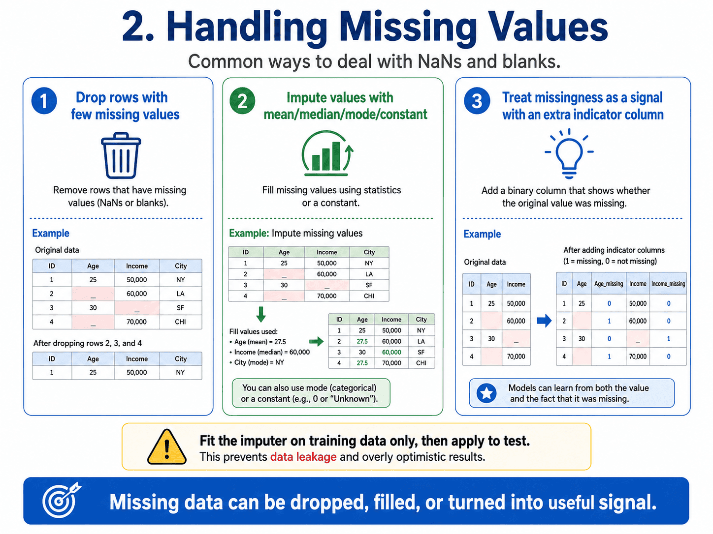
Treat "missing" as a signal. Sometimes the fact that a value is missing is itself informative. Add a "was-missing" indicator column alongside the imputed value.

from sklearn.impute import SimpleImputer
imputer = SimpleImputer(strategy='median')
X_train_filled = imputer.fit_transform(X_train)

A crucial detail. We fit the imputer on training data only, and apply it to the test.

Otherwise, we leak information (full coverage on Day 22: Data Leakage, ML Workflow & Interview Cheat Sheet).

3. Encoding Categorical Variables:

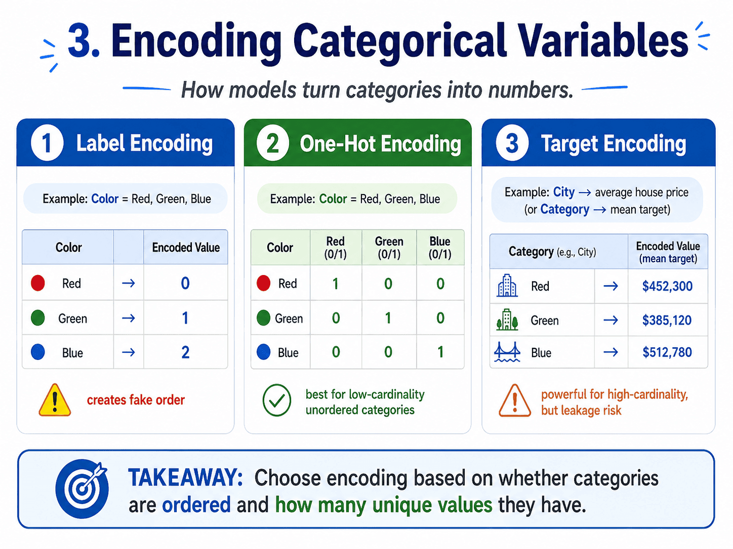
Models speak numbers. Categorical columns have to be translated.

Label Encoding. Red → 0, Green → 1, Blue → 2. Simple. But it creates a fake order: the model now thinks Blue (2) is "twice" Green (1), which is nonsense.

Use label encoding when the category is genuinely ordinal (small < medium < large), or for tree-based models, which do not mind.

One-Hot Encoding. Red → [1, 0, 0], Green → [0, 1, 0], Blue → [0, 0, 1]. Each category becomes its own binary column. No fake order.

Use it when categories are unordered AND the cardinality is small (under ~20).
Avoid it when cardinality is huge (cities, zip codes), because the feature count explodes.

Target Encoding. Replace the category with the mean of the target for that category. For example, "city → average house price in that city." Powerful for high-cardinality categoricals, but dangerous. Easy to leak target information if done outside cross-validation.

import pandas as pd
encoded = pd.get_dummies(df, columns=['color'])   # one-hot

4. Scaling Numerical Features:

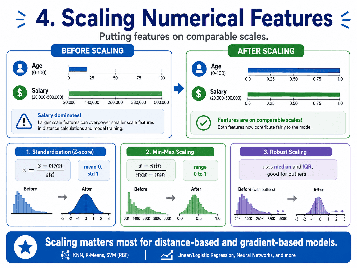
Imagine two features:

Age: range 0 to 100.
Salary: range 20,000 to 500,000.

A distance-based model (KNN, K-Means) will treat salary as much more important than age, just because the numbers are bigger. Scaling brings features onto comparable ranges.

Standardisation (Z-score).

z = (x − mean) / std

Each feature becomes mean 0 and std 1. This is the standard default. Use it when data is roughly Gaussian.

from sklearn.preprocessing import StandardScaler
scaler = StandardScaler()
X_train_scaled = scaler.fit_transform(X_train)
X_test_scaled = scaler.transform(X_test)   # use the SAME scaler

Min-Max Scaling.

x_scaled = (x − min) / (max − min)

Each feature is squashed into [0, 1]. Useful when features have hard bounds (image pixels 0–255) or for algorithms that assume bounded inputs.

Robust Scaling. Uses the median and the interquartile range instead of mean and std. Use it when outliers would skew the standard scaling.

5. Which Models Need Scaling? (Classic Interview Question):

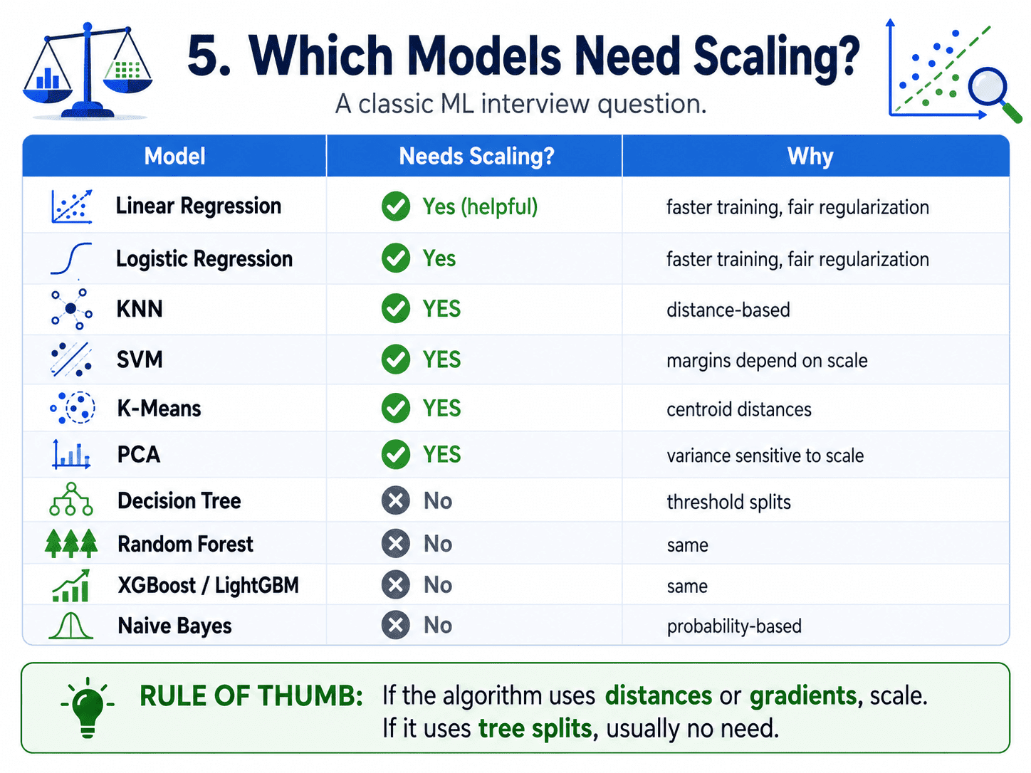
A rule of thumb worth remembering. If the algorithm uses distances or gradients, we scale. If it uses splits on individual features, we do not bother.

6. Handling Outliers:

An outlier is a row that is wildly far from the rest. Three approaches.

Remove the outlier if we can confirm it is an error.
Cap it (also called winsorising): set anything above the 99th percentile to the 99th percentile.
Transform it: log(x) shrinks the range of huge numbers (income, population).

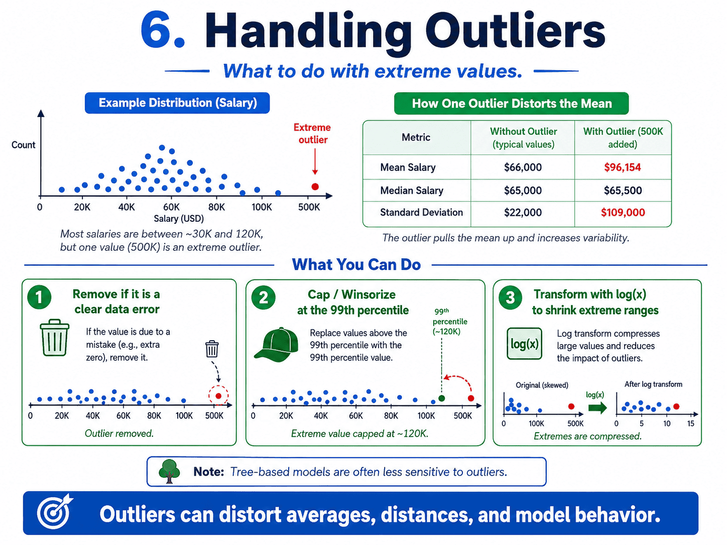
For example, on a salary column where most values lie between $30k and $200k but one row shows $50M (a CEO entry in a regular-employee table), the mean salary jumps by hundreds of thousands. Any distance-based model treats that one row as if it were ten neighbours of signal. Capping at the 99th percentile or applying log(salary) brings it back to a sane scale without throwing the data away.

Or use models that do not mind outliers. Tree-based models barely flinch.

7. Creating New Features:

This is the artisanal part of ML. Some examples that often help.

Ratios: debt / income, price / square foot.
Differences: days_since_last_purchase.
Interactions: temperature × humidity.
Datetime parts: split a timestamp into day of week, month, is_weekend.
Aggregations: average spend per customer over the last 30 days.
Binning: convert age into groups (0–18, 19–35, 36–60, 60+).

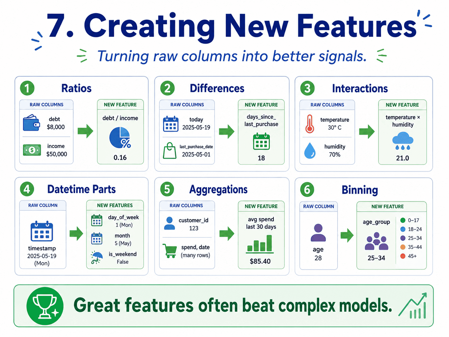
Good features encode the kind of reasoning a human would do about the problem. This is where domain knowledge really pays off.

8. The Full Pipeline:

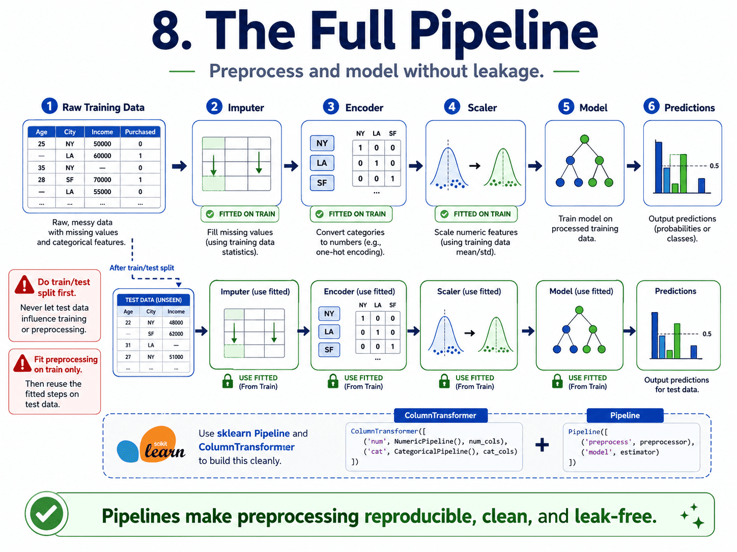
In real projects, we chain everything into a sklearn Pipeline so it runs identically on train and test.

from sklearn.pipeline import Pipeline
from sklearn.preprocessing import StandardScaler
from sklearn.linear_model import LogisticRegression

pipe = Pipeline([
    ('scaler', StandardScaler()),
    ('model', LogisticRegression())
])

pipe.fit(X_train, y_train)
pipe.score(X_test, y_test)

The pipeline learns the scaler on train, applies it to test, and trains the model, all in one call. Clean, reproducible, and leak-free.

A small thought to sit with. Suppose we have a "zip code" column with thirty thousand unique values. One-hot encoding would create thirty thousand columns.

What would we do?

A few options. We could target-encode it (replace each zip with the average target in that zip), carefully using cross-validation to avoid leakage.

We could group by geography (the first three digits of the zip = broader region) to reduce cardinality. Or we could use a tree-based model that handles high-cardinality categoricals better, or libraries like LightGBM and CatBoost that have native categorical support.

9. A Few Common Confusions Cleared:

Should I scale before or after train/test split? After. Fit the scaler on training data only, then apply to test. Scaling before would leak test info into training.
Is one-hot encoding always bad for high cardinality? Yes for linear models (too many features, too much sparsity). Tree-based models cope a bit better but still suffer.
What if a category appears in test but not train? Pick a strategy upfront. Either label it "Unknown," apply the overall average for target encoding, or use a model that handles unseen categories gracefully.
Why is target encoding risky? Because the encoding uses the target. If we compute it on the whole dataset, we have leaked future info into the features. Always compute it within cross-validation folds.
Common interview question: "Why does KNN need scaling but Decision Trees do not?" KNN uses distances, which are dominated by large-scale features. Decision Trees split each feature independently using thresholds, so the scale does not matter.

10. If This Came In An Interview:

A few questions to be ready for, with one-line answers.

Which models need feature scaling and which do not? Need: Linear / Logistic Regression, KNN, SVM, K-Means, PCA. Do not need: Decision Trees, Random Forest, Gradient Boosting, Naive Bayes.
Why does KNN need scaling but Decision Trees do not? KNN uses distance, so large-scale features dominate. Decision Trees split each feature using thresholds, where scale does not matter.
One-hot vs label vs target encoding? One-hot for unordered, low-cardinality categoricals. Label for ordinal categoricals or tree-based models. Target encoding for high-cardinality categoricals, but only within a CV loop to avoid leakage.
Should you scale before or after train/test split? After. Fit the scaler on training data only, then apply it to test. Otherwise we leak test statistics into training.
How do you handle missing values? Drop rows (if very few), impute with mean/median/mode/constant, or add a "was-missing" indicator column. The choice depends on the data.
What is target leakage? When a feature secretly contains information about the target, features that would not exist at prediction time. Often shows up as suspiciously high feature importance.
What is the difference between Standard, Min-Max, and Robust scaling? Standard makes mean = 0 and std = 1 (default). Min-Max squashes to [0, 1] (good when features have hard bounds). Robust uses median and IQR (good when outliers exist).
How would you handle a categorical feature with 30,000 unique values? Avoid one-hot (too sparse). Use target encoding within CV folds, or group by a broader category (zip → region), or use a model with native categorical support like LightGBM/CatBoost.

11. Summing It Up:

If we remember one thing from today, it is this: the best model on bad features will lose to a simple model on great features. Feature engineering is where most ML wins are won. We encode categoricals smartly, scale only when the algorithm cares about distances or gradients, treat missing values deliberately, and build features that capture human reasoning about the problem.

Coming Up on Day 9: Regularization — Ridge, Lasso, ElasticNet

We already met overfitting on Day 2: Train-Test Split & The Sin of Overfitting and the bias-variance seesaw on Day 3: Bias-Variance Tradeoff — Why Models Fail. Tomorrow we meet the most popular tool for controlling variance in linear models: Regularisation (Ridge, Lasso, ElasticNet). It is also the answer to one of the most asked interview questions, which is "how do you prevent overfitting in a linear model?"

That's all for today. Let's meet up again tomorrow with Day 9.

Thanks for reading.

Cheers!