Day 7: Gradient Descent — How Models Actually Learn

We have been saying "the model learns the best parameters" for six days now. Today we open that black box. Gradient Descent is the engine that powers nearly every modern ML algorithm, and the answer to one of the most common interview questions: "how does a model actually learn?"

This blog post is a daily learning summary of my ML self-study.

Terms Used Today

Gradient: The direction of steepest increase in the loss. We step the opposite way to make the loss smaller.

Learning rate: The step size at each update. Too big oscillates; too small crawls.

Loss surface: A 3D picture (or higher) of how loss changes with the model's parameters.

Epoch: One full pass through the training data.

Batch / Mini-batch / SGD: Different choices for how much data we use per update step.

Local minimum vs Global minimum: Gradient descent can sometimes get stuck in a small valley that is not the lowest one overall.

1. The Foggy Mountain:

Imagine we are standing on a mountain in thick fog. We cannot see the bottom. We just want to get down.

What do we do? We feel the slope under our feet. We take a small step in the steepest downward direction. Then we feel again. Step again. Eventually we reach the bottom.

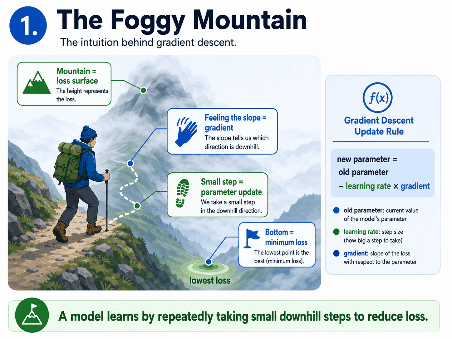
That is Gradient Descent in one paragraph. The whole algorithm. If we replace "mountain" with "loss surface," "bottom" with "smallest possible error," and "step direction" with "gradient," we have the textbook definition.

2. The Loss Surface:

On Day 4 we met our first loss function (MSE), and on Day 5 we met another one (log loss). The loss depends on the model's parameters (the beta values). If we plot it:

The x-axis is one parameter (β₁).
The y-axis is another parameter (β₂).
The z-axis (height) is the loss for those parameter values.

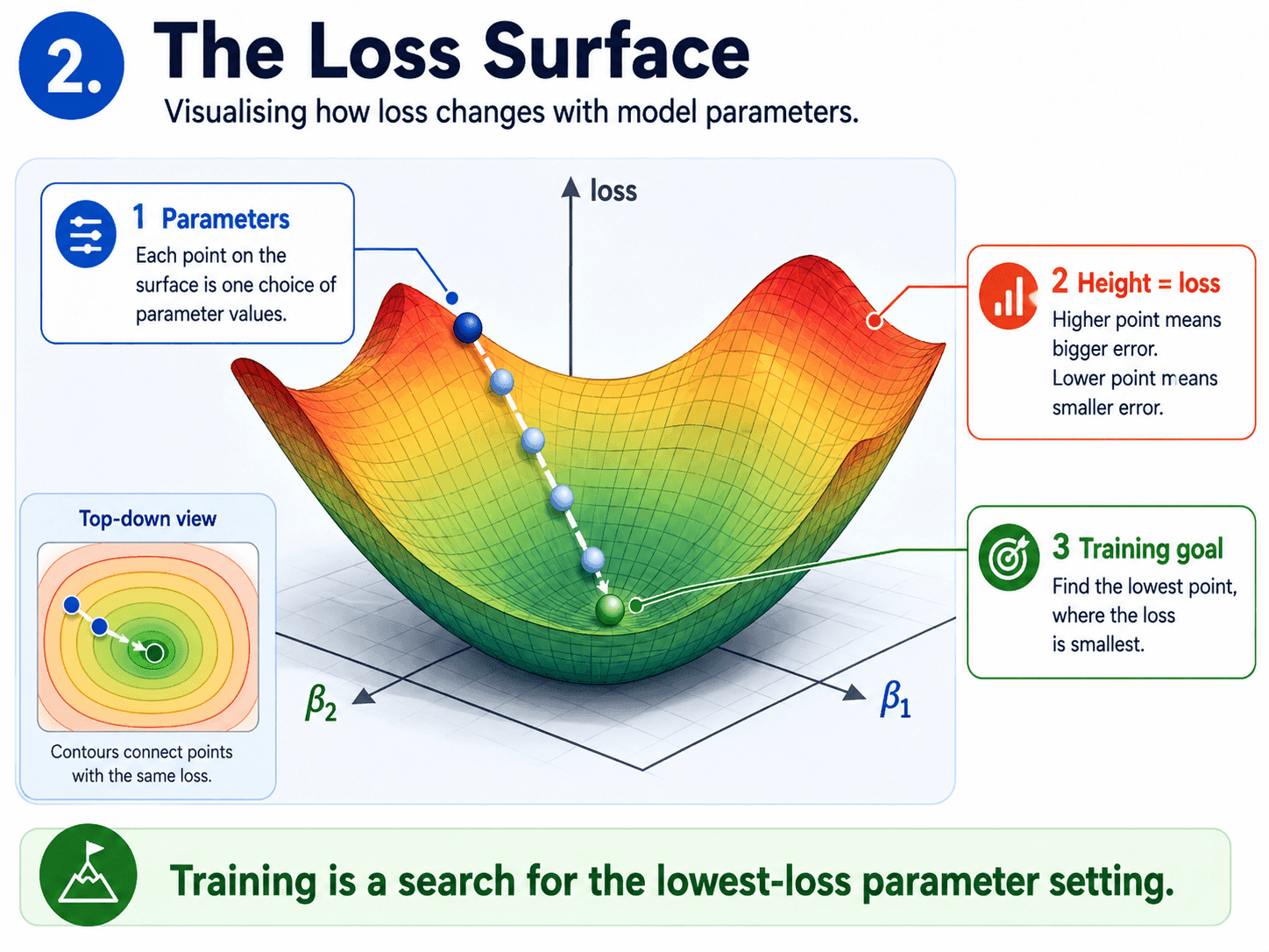
We get a 3D surface. Hills are bad (high loss). Valleys are good (low loss). The lowest point on the surface is the best our model can do. Training is the search for that lowest point.

3. The Update Rule:

At every step, Gradient Descent does this.

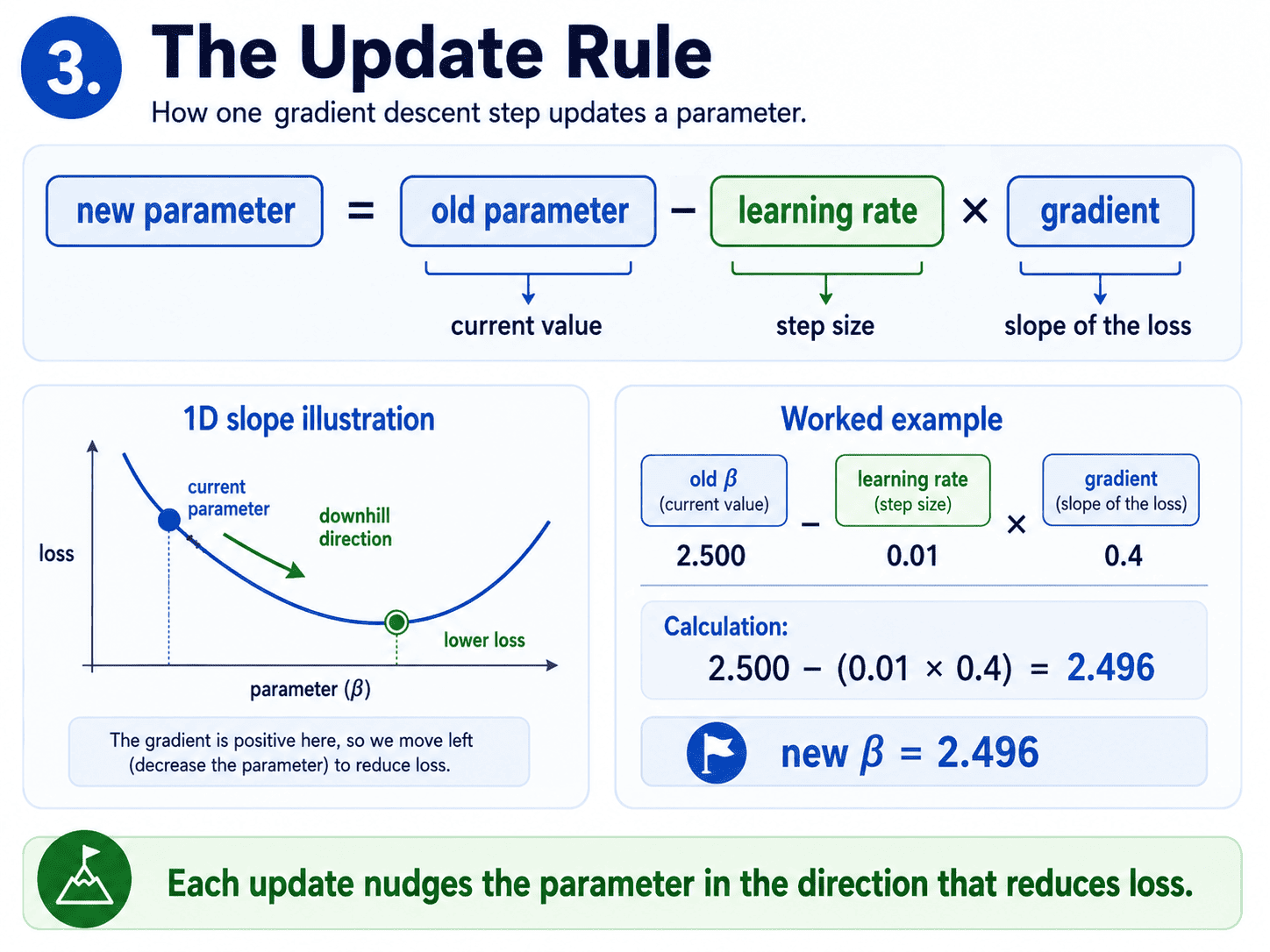
new parameter = old parameter − (learning rate × gradient)

In plain English:

The gradient tells us which way is uphill (toward bigger loss).
The minus sign flips that, so we go downhill.
The learning rate decides how big each step is.

Repeat until the loss stops dropping. That is it.

A tiny concrete example. Say our current parameter value is β = 2.500, the gradient at that point is 0.4, and the learning rate is 0.01. Then:

new β = 2.500 − (0.01 × 0.4) = 2.496

A small step in the right direction. Do this thousands of times, and the parameter ends up where the loss is smallest. Libraries handle the gradient maths for us. We just need to know what the update is doing.

4. The Learning Rate:

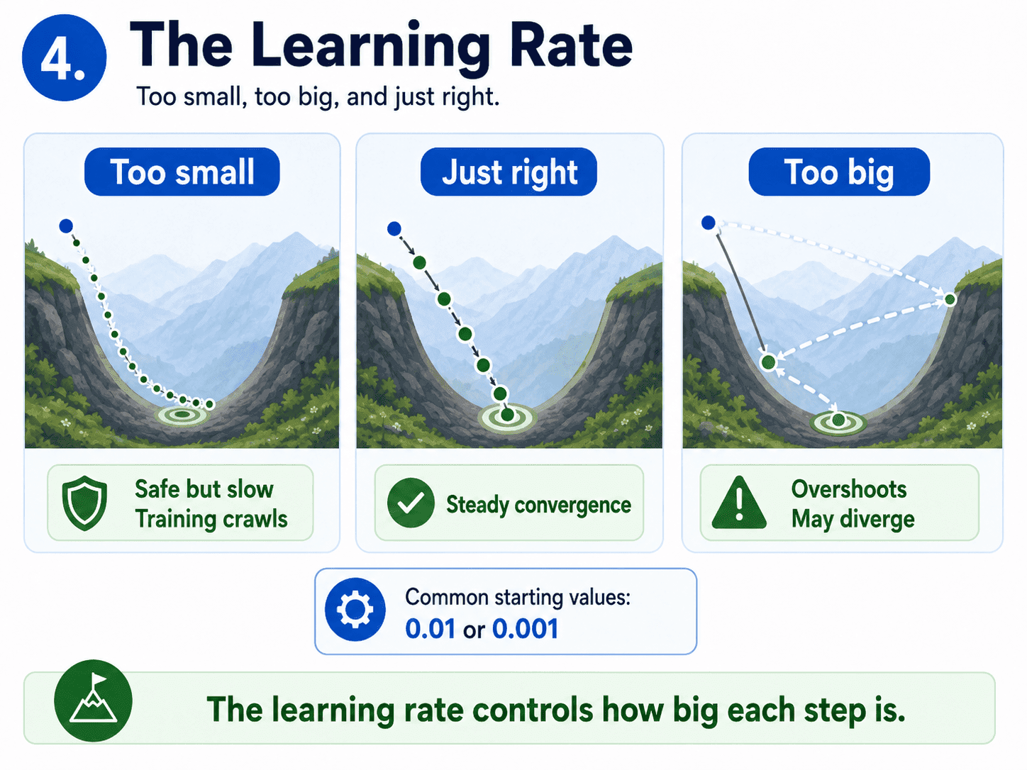
This is the most important single number in Gradient Descent, and the easiest one to get wrong.

Too small → tiny steps, training drags on forever, and we may stop before reaching the valley.
Too big → we overshoot the bottom and bounce around forever, or worse, the loss explodes to infinity.
Just right → smooth, steady descent into the valley.

Picture it visually. With a tiny learning rate, we crawl down the mountain, safe but slow. With a huge learning rate, we take giant leaps that overshoot the valley and land partway up the other side. Repeat.

We never converge. The sweet spot lies between these extremes.

Typical starting values in practice are 0.01 or 0.001, and we tune from there.

5. Three Flavors of Gradient Descent:

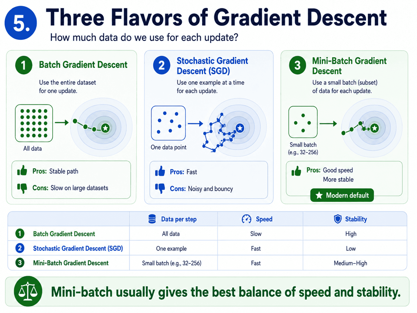
How much data do we use at each step? Three choices.

Batch Gradient Descent. Use all training data at every step. Compute the gradient over the entire dataset, then take one step.

Very stable, smooth path to the minimum.
Painfully slow on big datasets, because one step needs a full pass through millions of rows.

Stochastic Gradient Descent (SGD). Use one random training example per step.

Lightning fast.
The path is noisy and bouncy, like a drunk walking downhill.
Sometimes that noise actually helps by knocking the model out of bad local minima.

Mini-Batch Gradient Descent. The middle path. Use a small batch (say 32 or 64 examples) per step.

Faster than full batch, more stable than pure SGD.
This is the default in modern ML.

Almost every model we will train uses mini-batch under the hood, even when sklearn hides it from us.

6. Local Minima vs Global Minima:

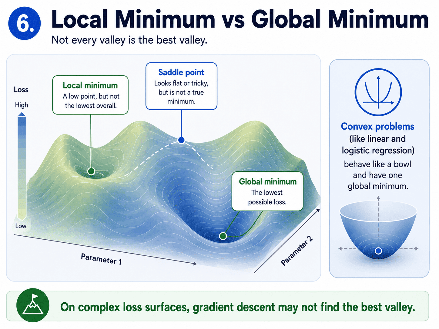
The loss surface is not always a smooth bowl. It can have:

A global minimum: the lowest possible point.
Local minima: small valleys that are not the lowest.
Saddle points: flat regions that look like minima but are not.

For Linear Regression and Logistic Regression, the loss surface is shaped like a bowl (this property is called convex), so Gradient Descent always finds the true minimum. For more complex models (gradient-boosted trees, neural networks), the surface is bumpy, and we might land in a local minimum. Tricks like momentum, the Adam optimiser, and clever initialisation help. We do not need the details today. Just know the landscape is not always friendly.

7. The Code:

Most algorithms hide Gradient Descent under the hood, but sklearn exposes it directly via SGDClassifier and SGDRegressor.

from sklearn.linear_model import SGDRegressor

model = SGDRegressor(learning_rate='constant', eta0=0.01, max_iter=1000)
model.fit(X_train, y_train)

Two key knobs:

eta0: the learning rate.
max_iter: the maximum number of passes through the data (epochs).

A fun small experiment. Set eta0 = 10 and watch the model explode. Set eta0 = 0.000001 and watch it crawl. It is the best way to feel the learning rate dial.

8. When We Will Actually Care About This:

Even though sklearn hides Gradient Descent for the most part, we will feel it any time:

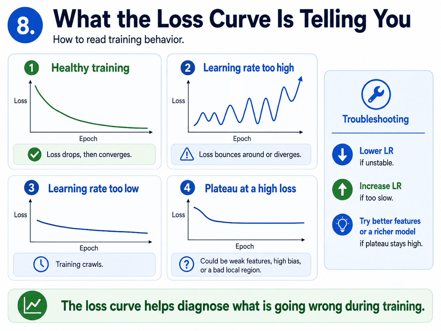
Training takes forever → maybe the learning rate is too small.
Loss bounces around or explodes to infinity → learning rate is too big.
Loss plateaus at a bad value → we are stuck in a local minimum, a saddle point, or the model is not expressive enough.
We move on to deep learning. Gradient Descent is its lifeblood.

A small thought to sit with. Suppose our loss curve drops fast for the first 50 epochs and then plateaus at a value that is still too high.

What might be happening?

It could be that the learning rate is too small to escape, we are at a local minimum or saddle, the model itself is not expressive enough (high bias, back to Day 3 Bias-Variance Tradeoff — Why Models Fail, or the features just are not informative enough.

First try increasing the learning rate or switching to a richer model. Diagnose, then act.

9. A Few Common Confusions Cleared:

Is Gradient Descent guaranteed to find the best answer? Only on convex problems (like Linear/Logistic Regression). Otherwise it finds a minimum, which may not be the minimum.
What is an "epoch"? One full pass through the training data. Models typically train for many epochs.
What are Adam, RMSprop, and Momentum? Smarter versions of Gradient Descent that adjust the learning rate automatically and remember past gradients. Adam is the safe default in deep learning.
Why subtract the gradient, not add? Because the gradient points uphill (toward bigger loss). We want to go downhill, so we subtract.
Most common interview question: "What is the learning rate, and what happens if it is too high or too low?" We now have the answer cold.

10. If This Came In An Interview:

A few questions to be ready for, with one-line answers.

How does gradient descent work? Start with random parameters. Compute the gradient of the loss. Take a small step in the opposite direction (downhill). Repeat until the loss stops dropping.
What is the learning rate? The step size at each update. Too small means training crawls. Too big means the loss oscillates or diverges.
What happens if learning rate is too high? Too low? Too high → loss bounces around or explodes to infinity. Too low → training is painfully slow and may never reach the minimum.
Batch vs Mini-batch vs SGD? Batch uses all training data per step (stable but slow). SGD uses one example per step (noisy but fast). Mini-batch uses a small batch (the modern default).
What is an epoch? One full pass through the training data. Models typically train for many epochs.
Local vs global minimum? A local minimum is a valley that is not the lowest one. For convex losses (Linear/Logistic Regression), there is only one minimum: the global. For non-convex losses, we may get stuck in a local one.
What is gradient descent's connection to boosting? Gradient boosting (XGBoost) is gradient descent in function space, where each new tree is a step downhill on the loss.
Why subtract the gradient instead of adding? Because the gradient points uphill (toward bigger loss). We want to go downhill, so we subtract.

11. Summing It Up:

If we remember one thing from today, it is this: a model learns by repeatedly nudging its numbers in the direction that lowers the loss. That is Gradient Descent. The learning rate sets the step size. Mini-batch is the modern default. Almost every model we ever train uses some flavor of it, even when it is hidden from view.

Coming Up on Day 8: Feature Engineering & Preprocessing

So far we have assumed our data arrives clean and ready to go. In real life, it never is. Tomorrow we tackle the most underrated skill in ML, the one that often matters more than the model choice itself: Feature Engineering and Preprocessing.

We will cover encoding categoricals, scaling numericals, handling missing values, and the answer to a beloved interview question: "which models need scaling and which do not?"

That's all for today. Let's meet up again tomorrow with Day 8.

Thanks for reading.

Cheers!