Day 6 Embeddings — Semantic Similarity, Cosine, and Dense vs Sparse

Day 5 wrapped up chunking and PDF processing. Today we go one layer deeper into embeddings themselves, the piece of the pipeline that actually decides which chunk is "closest" to a query. Retrieval is the day after.

Day 2 introduced embeddings with the meaning-map analogy. Today we go further. We will cover semantic similarity, cosine similarity, how nearest-neighbour search actually finds the top matches, and the difference between dense and sparse embeddings (and where TF-IDF and BM25 fit in).

This blog post is a daily learning summary of my 40 Day RAG class from Syed Jaffer of Parotta Salna.

Terms Used Today

Embedding: A list of numbers (a vector) that represents the meaning of a piece of text.

Vector space: The "map" where every embedding lives as a point or an arrow from the origin. It has hundreds of dimensions, not just the two we can draw on paper.

Semantic similarity: How close two pieces of text are in meaning, not in shared words.

Cosine similarity: A score from −1 to 1 that measures the angle between two embedding vectors. Higher = more similar.

KNN (K-Nearest Neighbours): Brute-force search for the K closest vectors to a query.

ANN (Approximate Nearest Neighbours): Smart-shortcut version of KNN. Almost as accurate, far faster at scale.

Dense embedding: A semantic vector where every dimension carries some meaning (used for similarity search).

Sparse embedding: A vector where most dimensions are zero (used for exact keyword matching, like BM25).

1. From Chunks to Vectors:

By the end of [[Day 5 Sliding Chunks, Token Costs & Processing Real PDFs|Day 5]] we had documents split into clean, well-sized chunks. The next job is to turn each chunk into something a vector database can actually search over: a list of numbers we call an embedding.

A small reminder. Embeddings are only relevant for vector-based RAG. If we are doing pure keyword search, we never embed anything. But almost every modern RAG pipeline is vector-based, because keyword search breaks the moment users phrase a question differently from the source text. Embeddings are how we get past that wall.

2. Semantic Similarity:

Search engines used to match words. Embeddings let us match meaning. That shift has a name: semantic similarity.

The classic example: king and queen. Different words, no overlapping letters, but they live in the same neighbourhood of meaning. Both royalty, both people. An embedding model places them very close together in the vector space.

Words and sentences with related meanings sit close to each other in this space. "Dog" sits near "puppy" and "wolf". "Doctor" sits near "nurse" and "hospital". A sentence like "my dog brings me joy" lands near "owning a pet improves happiness" even though they share almost no actual words.

When a user asks a question, we embed it, drop it into the same vector space, and look around for chunks that landed nearby. That nearness is what we mean by semantic similarity, and it is what makes RAG feel like the system actually understood the question.

3. Cosine Similarity:

Once we have two vectors in the same space, we need a number that says how close they are. The most common choice in RAG is cosine similarity.

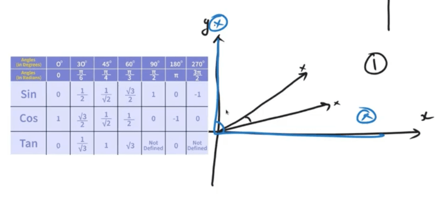
Imagine each embedding as an arrow shooting out from the origin. Cosine similarity asks one question: what is the angle between these two arrows?

A small angle (close to 0°) means the arrows point in almost the same direction. Cosine value is close to 1, very similar in meaning.
A right angle (90°) means the arrows are unrelated. Cosine value is 0.
Opposite directions (180°) mean they carry opposite meanings. Cosine value is −1.

The smaller the angle, the higher the cosine value, and the more similar the two texts are. That is why a similarity score of 0.92 between a query and a chunk is exciting, and 0.31 usually is not. Two more reasons cosine is the default. It ignores the length of the vectors. Only direction matters, so a one-line query can be compared fairly to a paragraph-long chunk. And it stays stable even when embeddings have hundreds or thousands of dimensions, where plain straight-line distance starts to lose meaning.

4. KNN and ANN:

Cosine similarity tells us how close two vectors are. But a vector database might hold millions of chunks. We need a way to find the top few nearest ones without scoring every single chunk against the query.

Two ideas show up here, and we only need the headline version of each.

KNN (K-Nearest Neighbours): Compare the query to every stored vector, then pick the top K closest. Simple, exact, and painfully slow once the index grows large.
ANN (Approximate Nearest Neighbours): Use a clever index that skips most of the obviously irrelevant vectors. We give up a tiny bit of accuracy and gain a huge speedup. Production vector DBs (FAISS, Pinecone, Chroma, Qdrant) all use ANN under the hood.

A small thought to sit with. When someone says "top-K retrieval", they almost always mean "top-K via ANN", not literally comparing the query to every vector in the database. The "approximate" part is doing a lot of work behind the scenes.

5. Symmetric vs Asymmetric Embedding Models:

Not all embedding models are built the same way. One important split is based on what kind of text they expect on each side of the comparison.

Symmetric models assume the query and the document look alike. Same style, similar length. Models like nomic-embed-text and Qwen3 embeddings sit in this camp. They are a good fit when you are matching sentences against sentences, or short paragraphs against short paragraphs.
Asymmetric models assume the query is short (a few words, often a question) and the document is long (a paragraph or full page). Models like Gemini's embedding model are trained for exactly this. The question side and the chunk side get encoded a little differently so they still line up correctly in the same space.

Match the model to the shape of your data. Symmetric for sentence-to-sentence search, asymmetric for short-question-to-long-document RAG, which is most real-world RAG.

6. Dense vs Sparse Embeddings:

The other big split is by what the vector looks like.

Dense embeddings are the semantic kind we have been discussing. Every dimension carries some meaning, most numbers are non-zero, and similarity is judged by direction in the space. Examples: OpenAI's text-embedding-3, Cohere Embed, and open-source models like the GPT-OSS 120B family. Dense embeddings are what you want when meaning matters more than exact words.
Sparse embeddings are the keyword kind. The vector has thousands of dimensions but almost all of them are zero. Only the words that actually appear in the text "light up". These are perfect when the match has to be exact: ISBN numbers, part IDs, serial numbers, error codes. A dense model will helpfully (and wrongly) decide that ISBN 978-3-16-148410-0 is "similar" to other long alphanumeric strings. A sparse model will only fire when those exact tokens appear.

For example,

A medical RAG over diagnosis notes → dense.
A spare-parts catalogue search → sparse.
A real-world product help-desk → usually both, blended together. That blend is called hybrid search, and it gets its own day later in the series.

7. A Quick Word on TF-IDF and BM25:

Sparse retrieval is older than dense retrieval, and a few classical terms are worth knowing because they still show up everywhere, including in OpenSearch and Elasticsearch.

TF (Term Frequency): how often a word appears in a document. The more often it shows up, the more "about" that word the document probably is.
IDF (Inverse Document Frequency): how rare the word is across the whole collection. Common words like the, is, of get downweighted because they appear everywhere. Rare words like thrombolysis or pgvector get boosted, because they actually distinguish one document from another.
BM25: the standard scoring formula that combines TF and IDF, with a couple of tweaks so a word appearing 100 times does not score 100× more than appearing once. BM25 is the workhorse behind OpenSearch and Elasticsearch keyword search to this day.

We do not need to memorise the formula. TF asks "does this word appear a lot here?", IDF asks "is this word rare enough to matter?", and BM25 mixes the two into one score.

8. A Small Demo with Ollama and ChromaDB:

Enough theory. Here is the smallest end-to-end demo. Embed a handful of sentences locally with Ollama, store them in ChromaDB, run a query, and then visualise the vector space using t-SNE.

import chromadb
import matplotlib.pyplot as plt
import numpy as np
import ollama
from sklearn.manifold import TSNE


def ollama_embed(texts):
    embeddings = []
    for t in texts:
        res = ollama.embeddings(model="nomic-embed-text", prompt=t)
        embeddings.append(res["embedding"])
    return embeddings


docs = [
    "Python is a programming language",
    "FastAPI is great for building APIs and mainly used in vector based solutions",
    "ChromaDB is a vector database",
    "I love machine learning",
    "PostgreSQL is a relational Database",
]

client = chromadb.Client()
collection = client.create_collection("ollama_demo")

emb = ollama_embed(docs)
collection.add(
    documents=docs,
    embeddings=emb,
    ids=[str(i) for i in range(len(docs))],
)

query = "tell me about vector database"
q_emb = ollama_embed([query])
results = collection.query(query_embeddings=q_emb, n_results=3)
print(results["documents"])

# Visualise the space
data = collection.get(include=["embeddings", "documents"])
embeddings = np.array(data["embeddings"])
documents = data["documents"]


def plot_embeddings(embeddings, labels, title):
    reducer = TSNE(n_components=2, perplexity=3, random_state=42)
    reduced = reducer.fit_transform(embeddings)

    plt.figure(figsize=(10, 7))
    plt.scatter(reduced[:, 0], reduced[:, 1], c="blue", edgecolors="k", alpha=0.6)
    for i, txt in enumerate(labels):
        plt.annotate(
            txt,
            (reduced[i, 0], reduced[i, 1]),
            fontsize=9,
            xytext=(5, 2),
            textcoords="offset points",
        )
    plt.title(f"Embedding Visualization using {title}")
    plt.grid(True)
    plt.show()


plot_embeddings(embeddings, documents, "t-SNE")

A few things worth noticing.

nomic-embed-text is a symmetric, dense embedding model. A sensible default for this demo, where queries and docs are both short sentences.
The query "tell me about vector database" shares almost no words with "ChromaDB is a vector database" and "FastAPI is great for building APIs and mainly used in vector based solutions", yet both rank at the top. That is semantic similarity in action.
t-SNE is a trick that squashes the hundreds-of-dimensions embedding down to 2D so we can actually see which sentences cluster together. The perplexity=3 is roughly how many neighbours t-SNE considers around each point. We keep it small here because we only have 5 sentences; on a real dataset, 30 is the usual default. The vector DB does not need this step. It is purely for our eyes.

A small but important point runs through every section above. Context is really important. Embeddings only know what the chunk gave them. If our chunks are noisy, broken mid-sentence, or stripped of surrounding meaning, even the best embedding model will miss the right answer. Good chunking from [[Day 3 Chunking — The Make-or-Break Decision in RAG|Day 3]] and [[Day 4 Semantic Chunking — When Meaning Decides Where to Split|Day 4]] is what makes today's embeddings shine.

9. If This Came In An Interview:

What is an embedding? A list of numbers that represents the meaning of a piece of text as a point in a vector space with many dimensions.
What is semantic similarity? Closeness of meaning between two texts, measured as nearness of their embeddings in the same vector space.
Why cosine similarity over Euclidean distance? Cosine measures the angle, ignores vector length, and stays stable in high dimensions. A better fit for comparing queries of different sizes against chunks.
What is the difference between KNN and ANN? KNN compares the query to every stored vector (exact, slow). ANN uses an index to skip most vectors (approximate, fast). Production vector DBs use ANN.
Symmetric vs asymmetric embedding models? Symmetric assumes the query and document look alike; asymmetric assumes a short query against a long document. Pick based on the shape of your data.
Dense vs sparse embeddings? Dense captures meaning (semantic search); sparse captures exact keywords (BM25, ISBNs, part IDs). Hybrid search uses both.
What is BM25? A scoring formula built on TF and IDF that ranks documents for keyword search; the default in OpenSearch and Elasticsearch.
Can I use one embedding model for the query and another for the documents? No. Different models live in different coordinate systems and will not line up.

10. Summing It Up:

If we remember one thing from today, it is this: embeddings turn text into vectors so that "similar meaning" becomes a real, measurable angle in space. Cosine similarity is how we measure that angle, ANN is how we search through millions of vectors quickly, and the choice between symmetric/asymmetric and dense/sparse decides whether retrieval feels right or weirdly off.

Coming Up on Day 7

We have prepared the chunks, embedded them, and stored them. Tomorrow we follow a single query end to end. From the raw question, through its embedding, through the vector DB's top-K search, and back as the context that finally goes into the LLM. We will also start peeking at the small but mighty tricks that lift retrieval quality, like re-ranking and hybrid search.

That's all for today. Let's meet up again tomorrow with Day 7.

Thanks for reading.

Cheers!