Day 5: Logistic Regression — When the Answer is Yes or No

Yesterday we fit a line to predict numbers. Today, we adapt that same idea for a different kind of question: yes or no. Logistic Regression is the workhorse of classification, and arguably the most important algorithm to know cold for an interview after Linear Regression.

This blog post is a daily learning summary of my ML self-study.

Terms Used Today

Sigmoid: An S-shaped function that squashes any number into the range (0, 1) so we can read the output as a probability.

Decision boundary: The line (or surface) the model uses to split predicted yes from predicted no.

Threshold: The probability cut-off (default 0.5) we use to convert a probability into a yes/no decision.

Log loss (binary cross-entropy): The loss function logistic regression minimises.

Linear classifier: A model whose decision boundary is a straight line, plane, or hyperplane.

Odds and log-odds: Ratios of probabilities that help us interpret the coefficients.

1. A Misleading Name:

First, the name. Logistic Regression is not regression. It does classification.

It is called "regression" because under the hood it borrows the linear regression machinery from Day 4. But the output is a probability, and we use that probability to assign a class. So the simplest one-line summary is this: Logistic Regression predicts probabilities, and then turns those probabilities into yes/no decisions.

2. The Problem Linear Regression Cannot Solve:

Imagine we want to predict whether a student passes an exam based on hours studied.

Hours studied	Passed?
1	0 (no)
3	0
5	1 (yes)
8	1

If we used Linear Regression directly, the line could slide right off the chart. It could predict 1.7 or even −0.4 for some inputs. Neither makes sense as a yes/no answer.

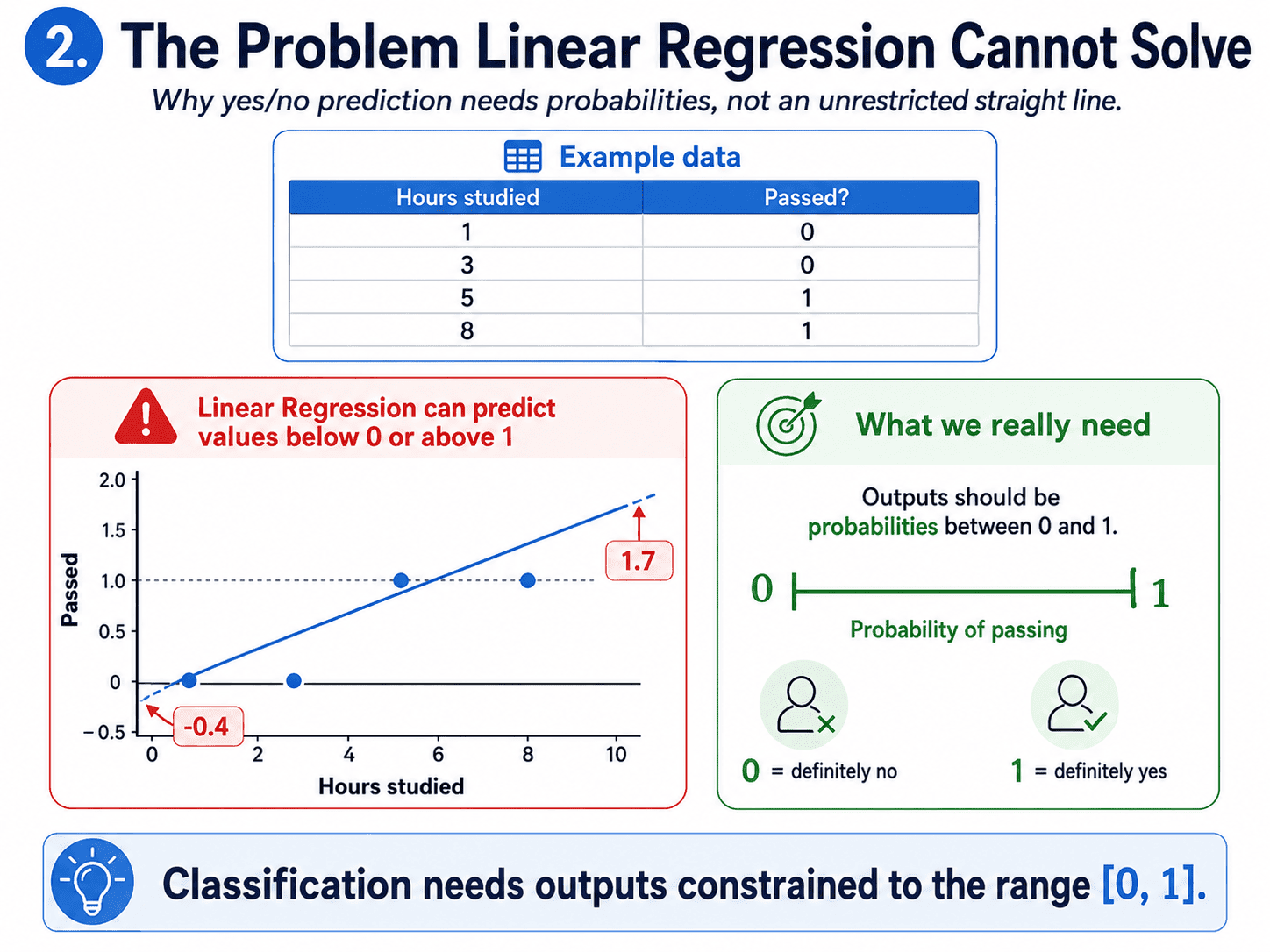
What we need is something that squeezes the output into the range [0, 1] so we can read it as a probability. That is exactly what the sigmoid function does.

3. Meet the Sigmoid Curve:

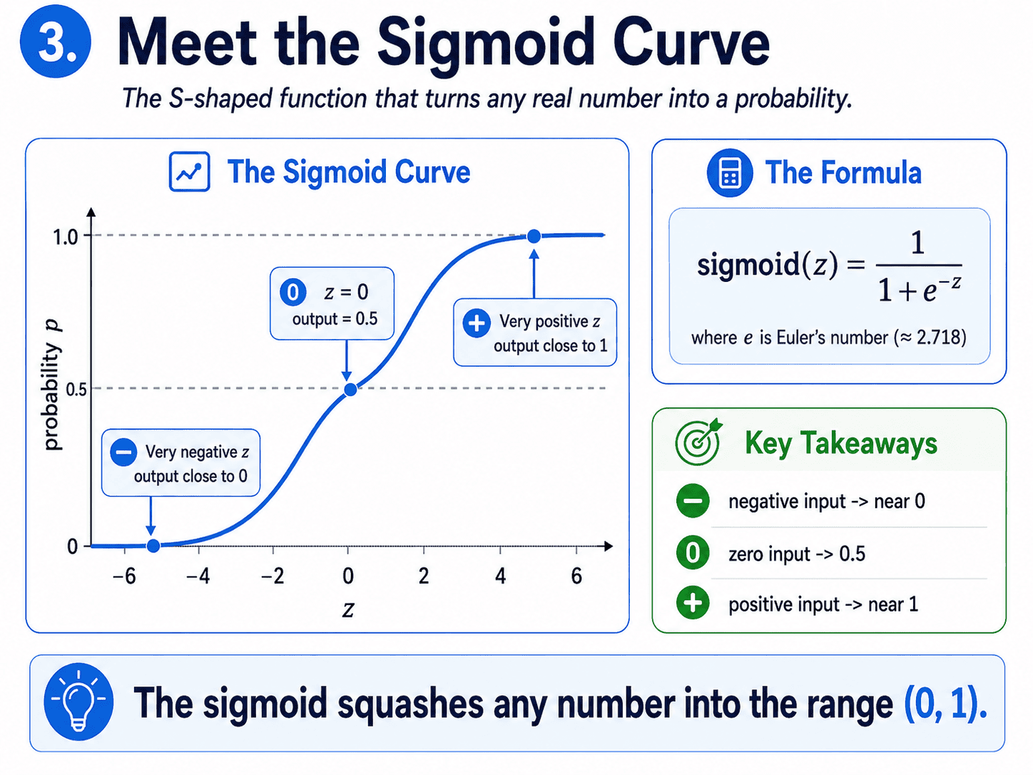
The sigmoid (also called the logistic function) takes any number and squashes it into the interval (0, 1).

sigmoid(z) = 1 / (1 + e^(−z))

We do not need to memorise the formula. The shape is what matters.

When z is very negative → output is close to 0.
When z = 0 → output is exactly 0.5.
When z is very positive → output is close to 1.

It looks like a stretched-out S. That S-curve is the heart of Logistic Regression.

4. How the Whole Thing Fits Together:

The full pipeline is just three steps.

Take the linear combination from [[Day 4 Linear Regression — Fitting the Best Line|Day 4]]: z = β₀ + β₁ · x₁ + β₂ · x₂ + ...
Push it through the sigmoid: p = sigmoid(z)
Read p as the probability that the answer is "yes."

Then we decide using a threshold. If p ≥ 0.5, predict yes. Otherwise, predict no.

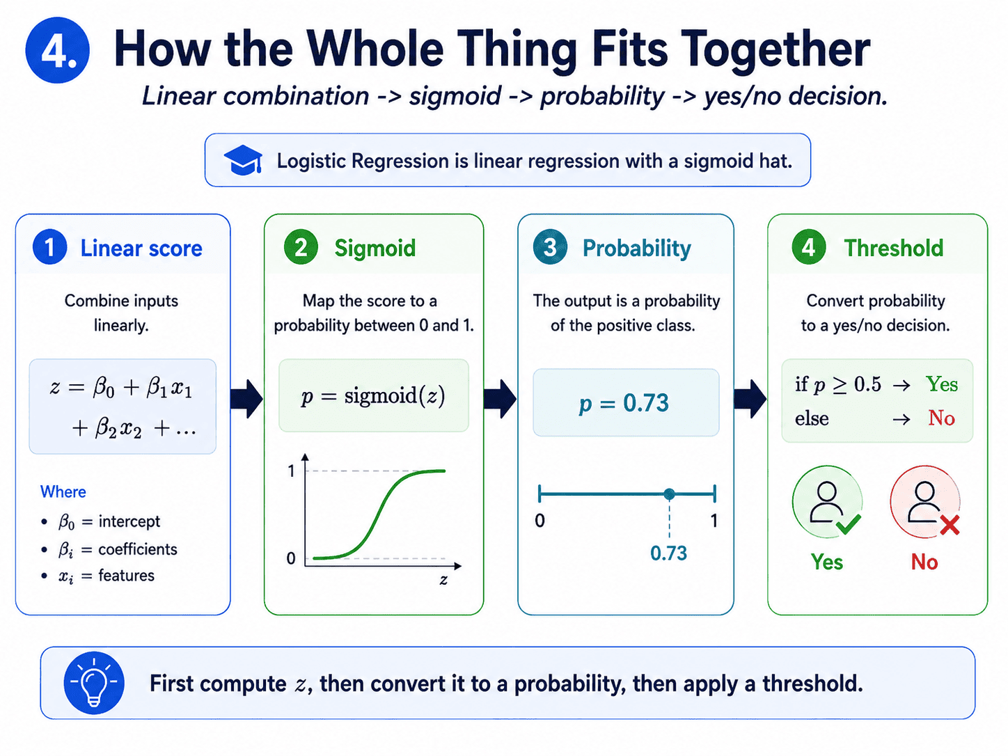So a Logistic Regression model is essentially the Linear Regression machine with a sigmoid hat on top.

5. The Decision Boundary:

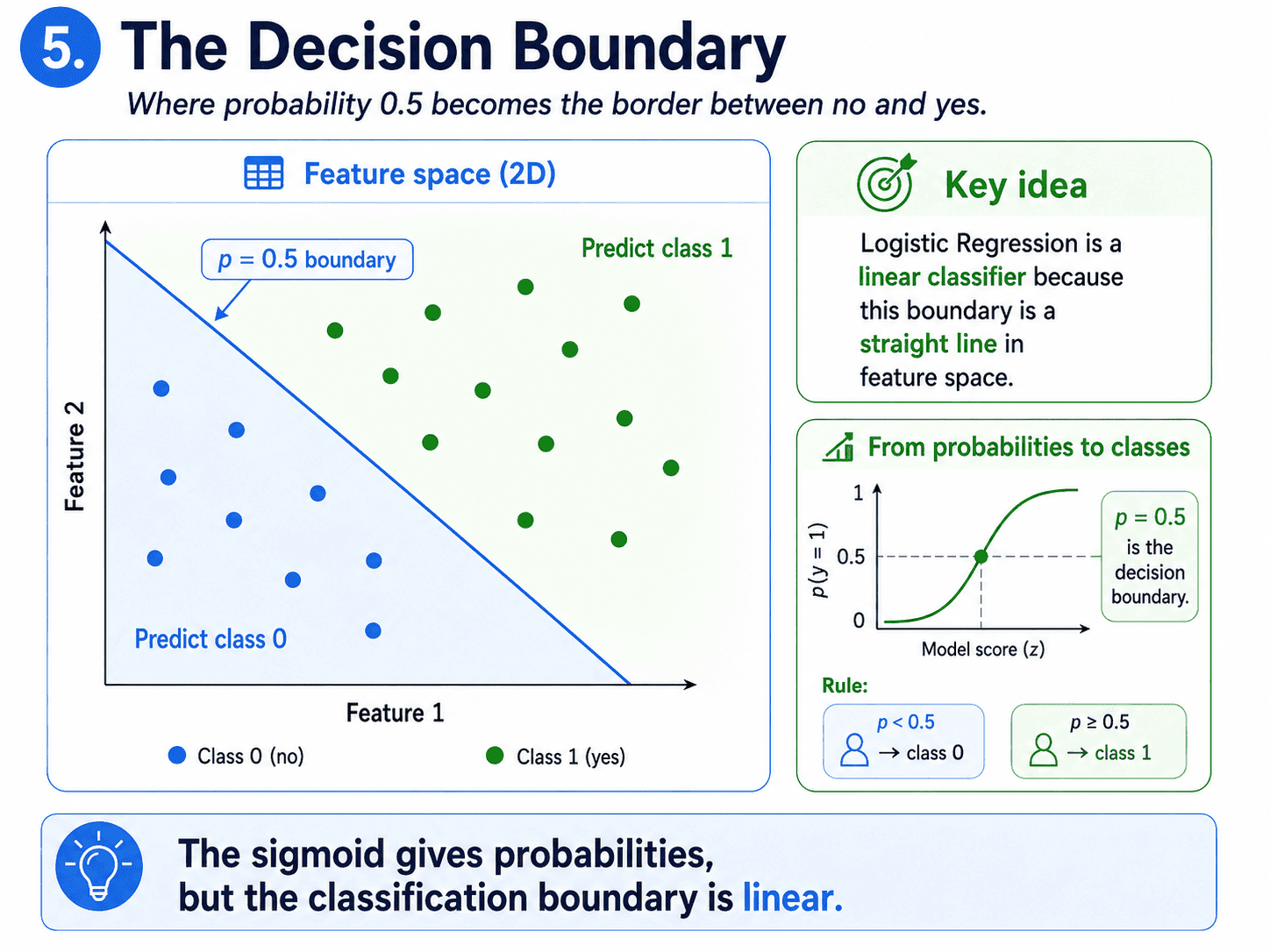
Here is a beautiful idea worth pausing on. Where the sigmoid outputs exactly 0.5, that is the boundary between yes and no. In feature space, that boundary is a straight line (or a flat plane in 3D, or a hyperplane in higher dimensions).

Logistic Regression draws a straight boundary between the two classes.

Anything on one side is predicted yes, and anything on the other side is predicted no. This is why Logistic Regression is called a linear classifier. The boundary is linear, even though the sigmoid output curve is not.

6. What "Training" Means Here:

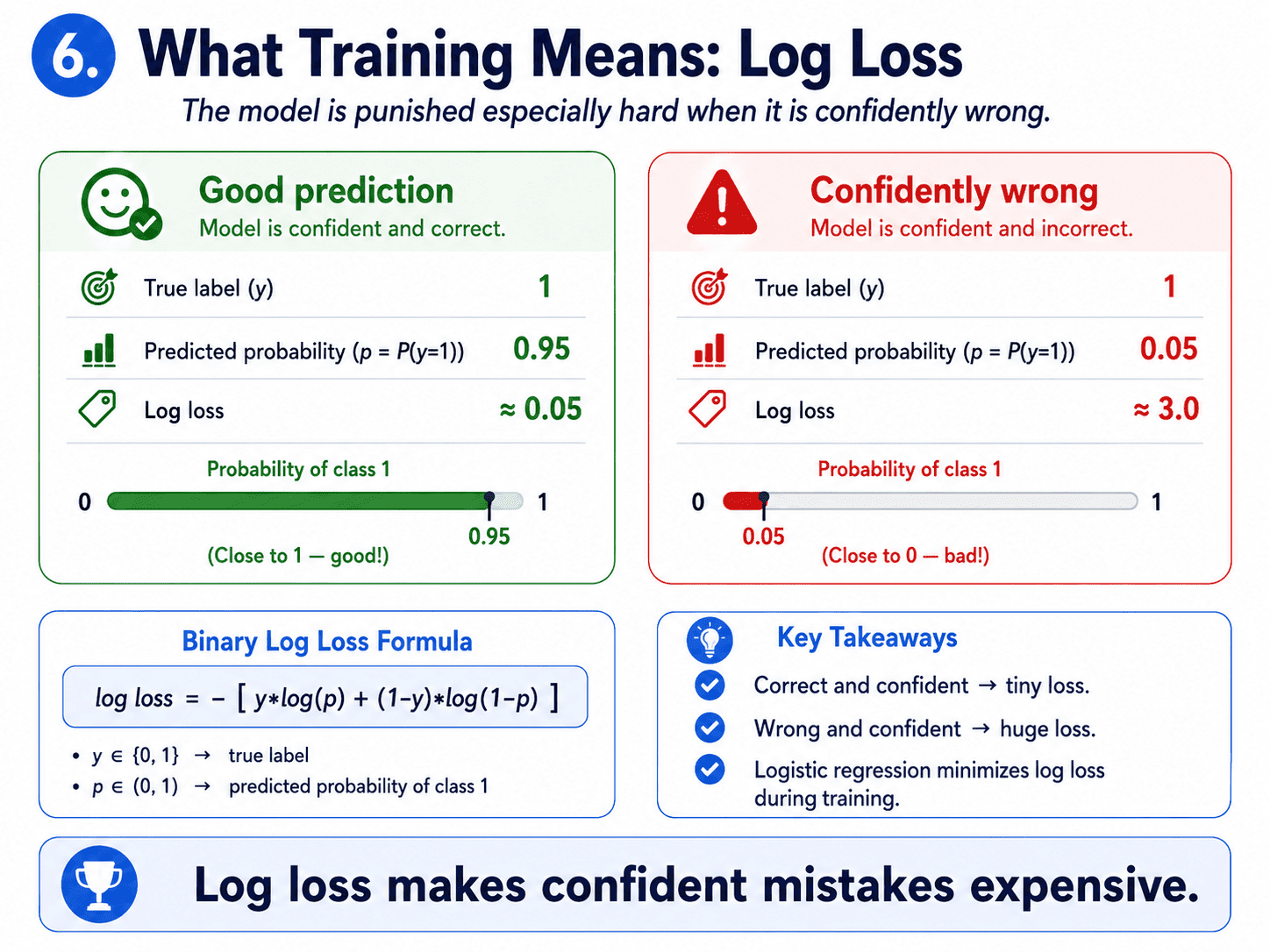
Linear Regression minimised MSE. Logistic Regression minimises a different loss called log loss (also called binary cross-entropy).

log loss = − [ y · log(p) + (1 − y) · log(1 − p) ]

No need to memorise the formula. The intuition is simple.

If true answer is 1 and we predicted close to 1 → loss is tiny.
If true answer is 1 and we predicted close to 0 → loss is huge.
The loss punishes confident wrong predictions especially hard.

A quick number check. If the true answer is 1 and we predict 0.95, log loss ≈ −log(0.95) ≈ 0.05 (tiny). If we predict 0.05 instead (very confidently wrong), log loss ≈ −log(0.05) ≈ 3.0 (huge).

That is roughly 60× the punishment for the same magnitude of confidence, just in the wrong direction. Now we see why "confidently wrong" is so painful for the model.

The optimiser (gradient descent, which we will meet on Day 7 on Gradient Descent — How Models Actually Learn tweaks the beta values to make this loss as small as possible.

7. The Code:

from sklearn.linear_model import LogisticRegression

model = LogisticRegression()
model.fit(X_train, y_train)

predictions = model.predict(X_test)             # 0 or 1
probabilities = model.predict_proba(X_test)     # probability per class
print(model.coef_, model.intercept_)

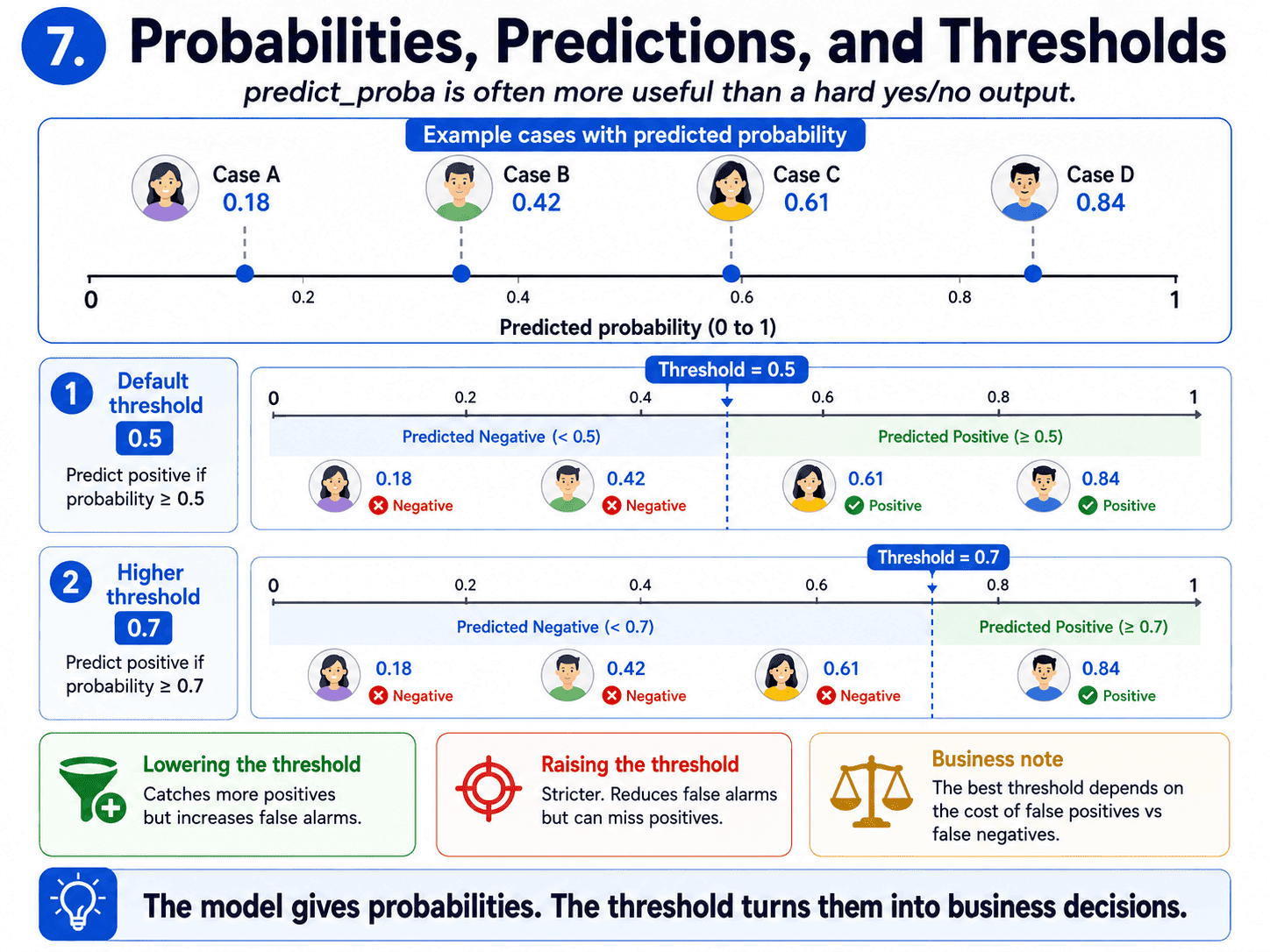
A small but important note. predict_proba is often more useful than predict. If we want fewer false alarms, we raise the threshold above 0.5. If we want to catch more true positives, we lower it.

We will see this dial again on Day 11 on Class Imbalance — Why Accuracy Lies when class imbalance forces us to tune the threshold.

8. Multi-Class? No Problem:

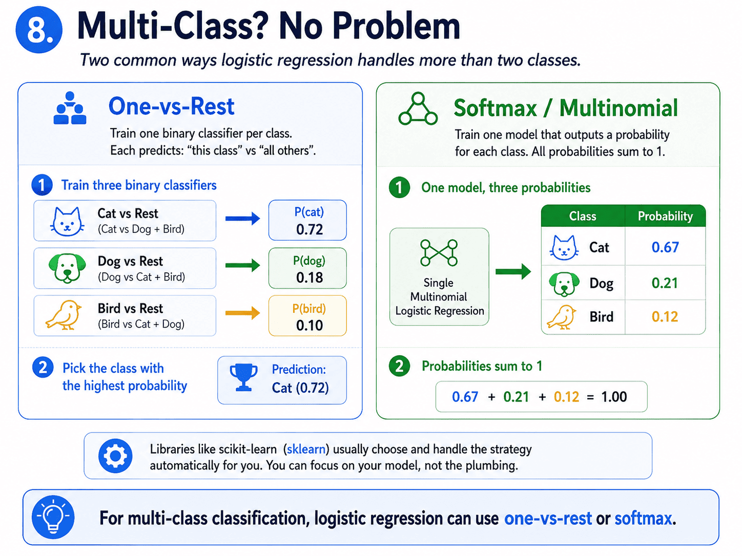
What if we have three or more classes (cat, dog, bird)? Two common tricks.

One-vs-Rest: Train one Logistic Regression per class, asking "is this a cat or not?", "is this a dog or not?", etc. Pick the class with the highest probability.
Softmax (Multinomial): A generalisation of the sigmoid that outputs one probability per class, all summing to 1.

sklearn picks the right approach for us automatically. We do not have to do anything beyond passing in a multi-class y vector.

9. What Coefficients Mean Here:

Coefficients in Logistic Regression are interpretable, but in a slightly different language than in Linear Regression. A positive coefficient means that increasing that feature increases the odds of class 1. The relationship is not as clean as "each extra sq ft adds $150," but it is still useful, and miles better than a black-box model.

10. When Logistic Regression Wins, When It Loses:

It wins when the classes are roughly linearly separable, when we need probabilities (not just hard labels), when interpretability matters (medical, legal, credit risk), and when we want a fast, strong baseline before reaching for anything fancier. It is the go-to first model for any binary classification problem.

It loses when the boundary between classes is curvy (circles within circles), when feature interactions matter a lot, or when we have many irrelevant features without regularisation. For curvy boundaries, decision trees and SVMs with kernels (coming later this series) do a much better job.

A small thought to sit with. If Logistic Regression outputs a probability of 0.6 for a customer churning, the manager wants a single "churn / no churn" decision. Why does the threshold matter? Because the threshold is a business decision, not a math one. If acting on a false positive is cheap (sending an email), we lower the threshold to 0.3 to catch more churners. If acting on a false positive is expensive (giving a discount), we raise the threshold to 0.7 to be more sure. The same model can serve very different purposes depending on the threshold we pick.

11. A Few Common Confusions Cleared:

Why is it called "regression" when it does classification? Because under the hood, it regresses (linearly combines features) onto the log-odds of the outcome. Old statistics name, stuck.
Why log loss and not MSE? With sigmoid plus MSE, the loss surface has flat regions where gradient descent stalls. Log loss has a much friendlier shape that learns faster and ends up at better minima.
Do I need to scale features? Yes, both for faster training and so that regularisation (Day 9 on Regularization — Ridge, Lasso, ElasticNet applies fairly across features.
Is the decision threshold always 0.5? No, that is just the default. We adjust it based on the business cost of false positives vs false negatives.
Common interview question: "Why is Logistic Regression a linear model?" Because the decision boundary is linear in the features. The non-linear sigmoid is applied only after the linear combination, to convert the result into a probability.

12. If This Came In An Interview:

A few questions to be ready for, with one-line answers.

Why is it called Logistic Regression if it does classification? Historical naming. It "regresses" features onto the log-odds of the outcome, then converts to a probability with the sigmoid.
Why is it a linear model? Because the decision boundary it draws between classes is linear in the features. The sigmoid only converts the output to a probability.
What loss does it minimise and why not MSE? Log loss (binary cross-entropy). MSE with sigmoid gives a non-convex surface with flat regions that make gradient descent stall.
What does adjusting the threshold do? Trades precision for recall. Lower threshold catches more positives but more false alarms. Higher threshold is stricter.
How do you handle multi-class? One-vs-Rest (one model per class) or Multinomial/Softmax (one model that outputs a probability per class summing to 1).
Does it need feature scaling? Yes. For faster training and so regularisation applies fairly across features.

13. Summing It Up:

If we remember one thing from today, it is this: Logistic Regression is Linear Regression with a sigmoid hat. The line gives us a number, the sigmoid turns it into a probability, the threshold turns it into a yes or no. Fast, interpretable, and the right first model for any binary classification problem.

Coming Up on Day 6 Evaluation Metrics — How Do We Know a Model is Good

So far, we have built two models and judged them with "score" or "accuracy" without thinking much about it. Tomorrow we take that question seriously. We will see why accuracy alone can mislead, and we will meet the metrics every interviewer expects us to know: precision, recall, F1, ROC-AUC, MAE, MSE, R², and friends.

That's all for today. Let's meet up again tomorrow with Day 6.

Thanks for reading.

Cheers!