Day 5: Sliding Chunks, Token Costs & Processing Real PDFs

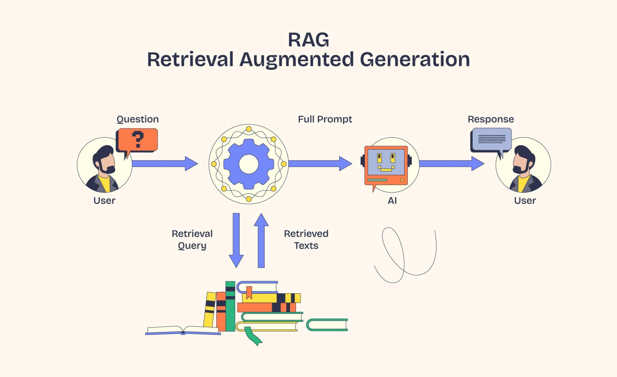
Day 4 promised PDF processing for today. Before we get there, two more chunking flavours worth meeting first. Sliding chunking and token-based chunking. Then we finally crack open a real PDF.

This blog post is a daily learning summary of my 40 Day RAG class from Syed Jaffer of Parotta Salna.

Terms Used Today

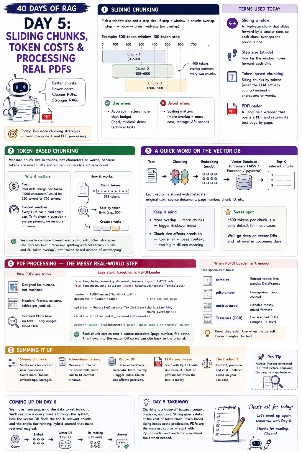
Sliding window: A fixed-size chunk that slides forward by a smaller step, so each chunk overlaps the previous one.

Step size (stride): How far the window moves forward each time.

Token-based chunking: Sizing chunks by tokens (what the LLM actually counts) instead of characters or words.

PyPDFLoader: A LangChain wrapper that opens a PDF and returns its text page by page.

OCR (Optical Character Recognition): Turning images of text (like scanned PDFs) into actual machine-readable text.

1. Sliding Chunking:

Sliding chunking is the close cousin of overlapping chunking from [[Day 3 Chunking — The Make-or-Break Decision in RAG|Day 3]]. We pick a window size and a step size. If the step is smaller than the window, chunks overlap. If they are equal, we are back to plain fixed-size with no overlap.

For example, a 500-token window with a 100-token step produces chunks at positions 0–500, 100–600, 200–700, and so on. Four hundred tokens are shared between every two chunks. A safety net for context near boundaries.

The catch is cost. Heavy overlap means we are storing the same tokens four or five times over. More embeddings, more storage in the vector DB, more money on paid APIs. Use sliding chunking when accuracy matters more than budget (legal, medical, dense technical text). Avoid it when scaling matters.

2. Token-Based Chunking:

Token-based chunking is less of a separate strategy and more of a discipline. It says: measure chunk size in tokens, not characters or words, because tokens are what LLMs and embedding models actually count.

Why does it matter? Two reasons.

Cost. Paid APIs charge per token. A "1000-character" chunk could be 250 tokens or 700 tokens depending on the content. Token-based sizing keeps the bill predictable.
Context windows. Every LLM has a hard token cap. To fit a chunk plus the question plus the system prompt inside that window, we have to measure in tokens.

We usually combine token-based sizing with one of the other strategies. The right phrase is "recursive splitting with 500-token chunks and 50-token overlap," not "token-based chunking instead of overlapping."

3. A Quick Word on the Vector DB:

We chunk the text, embed each chunk into a vector, and store it in a vector database (Chroma, FAISS, Pinecone, pgvector). Each vector is stored alongside metadata like the original chunk text, the source document, the page number, and a chunk ID. At query time, the user's question is also embedded, and the vector DB returns the top-K nearest chunks.

Two things to keep in mind. More overlap means more chunks, which means a bigger and slower index. And the chunk size affects retrieval precision. Too small loses context, too big dilutes meaning. The 500-token sweet spot exists for a reason. We will give vector DBs and retrieval their own days later, but this is enough to know what we are building toward.

4. PDF Processing:

PDFs were designed to look right when printed, not to be machine-readable. Headers, footers, columns, and tables all get jumbled when we extract raw text. And if the PDF is scanned, there is no text at all, just images of text that need OCR first.

For most clean text PDFs, LangChain's PyPDFLoader is the easiest start.

from langchain_community.document_loaders import PyPDFLoader
from langchain.text_splitter import RecursiveCharacterTextSplitter

loader = PyPDFLoader("handbook.pdf")
documents = loader.load()                                  # one doc per page

splitter = RecursiveCharacterTextSplitter(chunk_size=500, chunk_overlap=50)
chunks = splitter.split_documents(documents)

print(f"Loaded {len(documents)} pages, split into {len(chunks)} chunks")

Each chunk carries both the text and the source metadata (page number, file path), which flows into the vector DB and lets us cite results back to the original document.

When PyPDFLoader is not enough, there are specialised libraries worth knowing. camelot for extracting tables into pandas DataFrames, pdfplumber for fine-grained layout control, unstructured for messy mixed formats, and Tesseract for OCR on scanned documents. We do not need to memorise these. We just need to know they exist and reach for them only when the default loader mangles the text.

5. If This Came In An Interview:

What is sliding chunking? Fixed-size chunks that slide forward by a smaller step, so each chunk overlaps the previous one. Trades storage and cost for safer context across boundaries.
Why prefer tokens over characters for chunk size? Tokens are what LLMs and embedding models actually count. Character counts can wildly mislead (a "1000-character" chunk can be 250 or 700 tokens).
When should sliding chunking be avoided? When scaling matters, since heavy overlap multiplies embedding cost and storage.
Why is PDF processing tricky? PDFs were designed for printing, not parsing. Headers, footers, columns, and tables get jumbled. Scanned PDFs have no text at all, only images, and need OCR.
What do you reach for when PyPDFLoader is not enough? camelot for tables, pdfplumber for fine layout control, unstructured for messy mixed formats, Tesseract for OCR on scanned PDFs.

6. Summing It Up:

If we remember one thing from today, it is this: chunking is a tradeoff between context, precision, and cost. Sliding gives us safety nets at the cost of token bloat. Token-based sizing keeps the bill predictable. And PDFs, the messiest source of all, are usually a PyPDFLoader plus a careful look at the output, with camelot, OCR, or pdfplumber waiting in reserve for the harder cases.

Coming Up on [[Day 6 Embeddings — Semantic Similarity, Cosine, and Dense vs Sparse|Day 6]]

Five days of data prep is enough scaffolding. Tomorrow we step back into embeddings and go one layer deeper. Semantic similarity, cosine in more depth, a peek at how the vector DB actually finds the top matches at scale (KNN versus ANN), the split between symmetric and asymmetric models, dense vs sparse embeddings, and a small Ollama + Chroma demo to tie it all together. Retrieval itself gets its own deep dive in a later day.

That's all for today. Let's meet up again tomorrow with Day 6.

Thanks for reading.

Cheers!