Day 4 Linear Regression — Fitting the Best Line

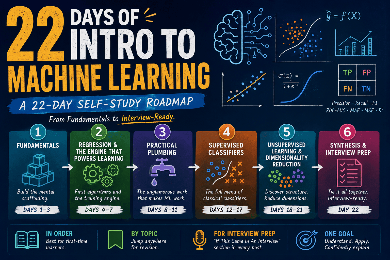
Three days of fundamentals and we are finally meeting our first real algorithm. Linear Regression is the simplest, oldest, and still one of the most used models in industry. It is also the model every interviewer expects us to know cold, because so many later ideas (regularisation, gradient descent, the very notion of a loss function) sit on top of it.

This blog post is a daily learning summary of my ML self-study.

Terms Used Today

• Linear regression: Finding a straight-line relationship between features and a numeric target.
• Coefficient (β): The multiplier on a feature; tells us how much the prediction changes per unit of that feature.
• Intercept (β₀): Where the line crosses the y-axis when all features are zero.
• Loss function: A formula that measures "how wrong" the model is. Training a model always means making this number as small as possible.
• MSE (Mean Squared Error): The loss function linear regression minimises. The average of (actual − predicted) squared.
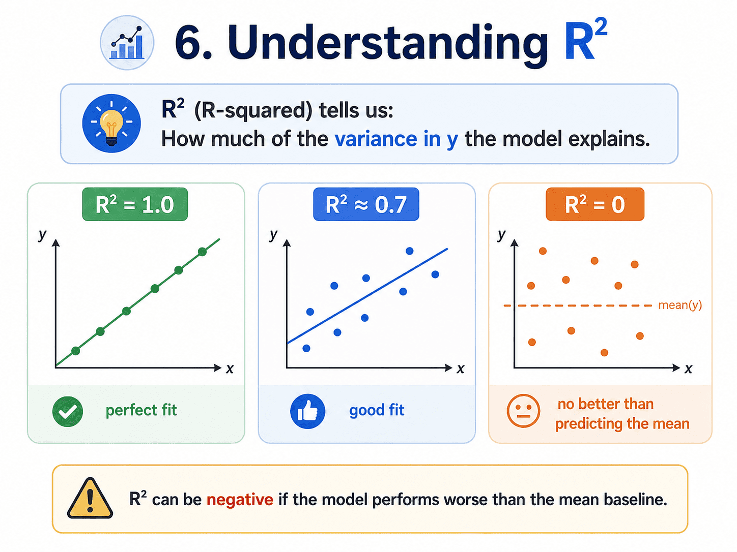
• R² (R-squared): Fraction of the variance in y the model explains. 1.0 is perfect, 0 is no better than predicting the mean.

1. The Setup:

Suppose we are looking at house prices.

Size (sq ft)	Price ($)
800	150,000
1200	220,000
1500	270,000
2000	360,000

Someone asks, "What is a 1700 sq ft house worth?" Most of us would look at the trend, mentally draw a line through the dots, and read off the answer. That is exactly what Linear Regression does, except more rigorously.

The whole idea is to draw the best straight line through our data and use it to make predictions for new points.

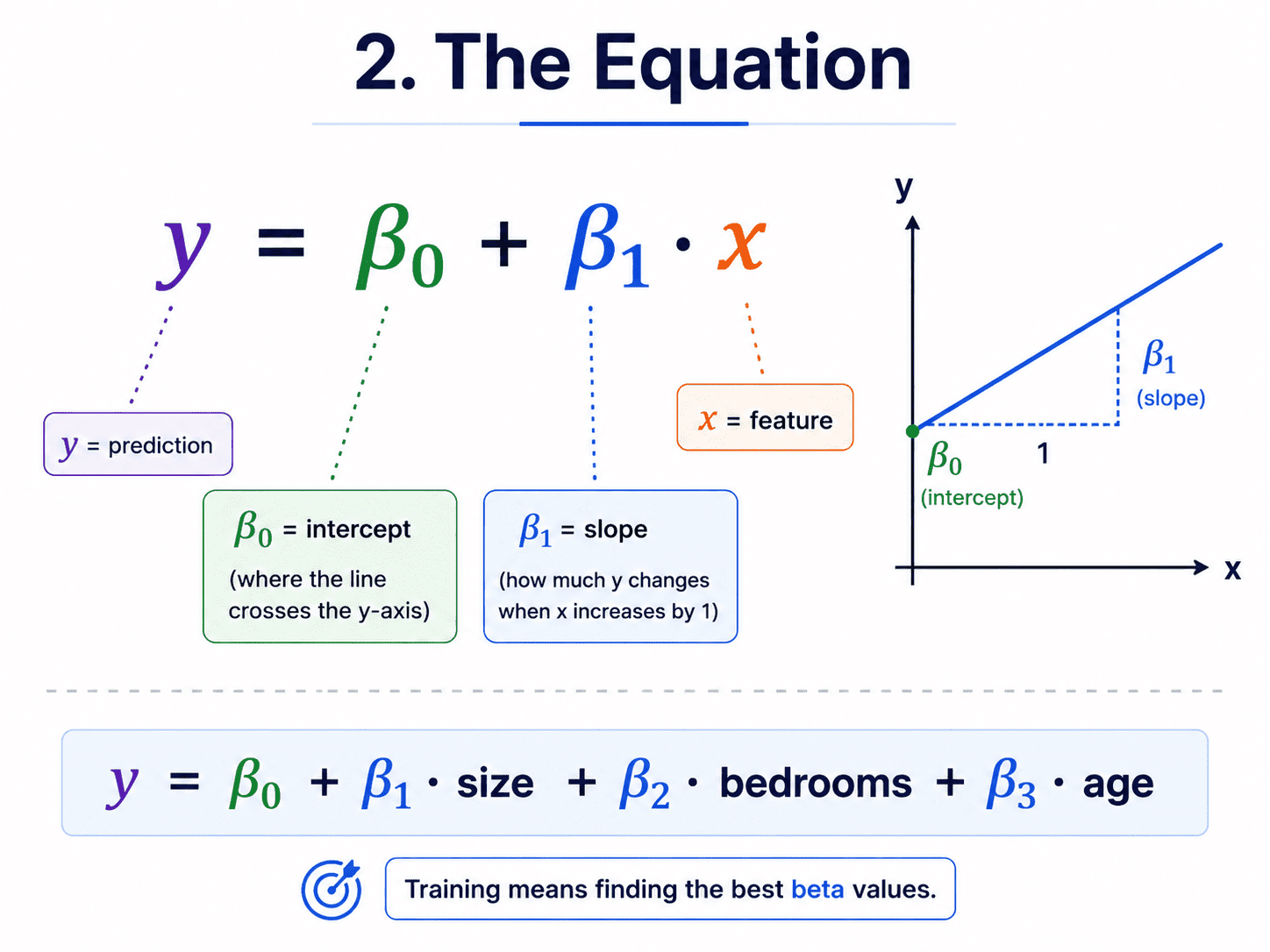
2. The Equation:

For a single feature, the model is the line we learned at school.

y = mx + b

In ML language, we usually write it as:

y = β₀ + β₁ · x

• β₀ (beta-zero, the intercept): where the line crosses the y-axis.
• β₁ (beta-one, the slope): how much y changes per unit of x.

For multiple features (say size, bedrooms, and age of the house), the equation just grows.

y = β₀ + β₁ · size + β₂ · bedrooms + β₃ · age

That is all. The whole "model" is a list of beta values. Training the model means finding the beta values that fit our data best.

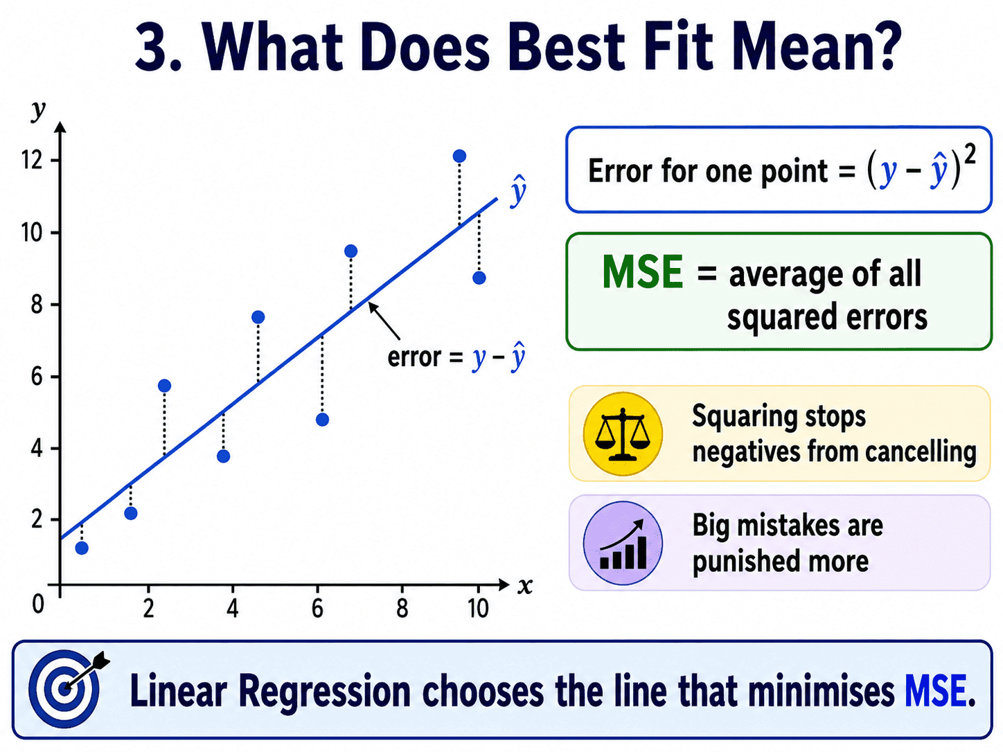
3. What Does "Best Fit" Mean?

Yesterday we said learning is just reducing error. Linear Regression is the cleanest example of that idea. For each point, the error is the gap between the actual y and the model's prediction ŷ. We square it before adding things up.

Error for one point = (y − ŷ)²

We square it for two reasons. First, so that negatives do not cancel positives. Second, so that big mistakes are punished more than small ones.

When we sum these squared errors across all training points and divide by the count, we get the Mean Squared Error, or MSE. Linear Regression finds the line that minimises MSE.

Training the model = minimising the squared errors.

This is the first time we are meeting the idea of a loss function. A loss function is just a formula that measures how wrong the model currently is. Every algorithm from here on has one. Logistic Regression uses log loss. Decision Trees use Gini. Training a model always means finding the parameters that make the loss as small as possible. If we hold on to this single sentence, much of the next eighteen days will tie together.

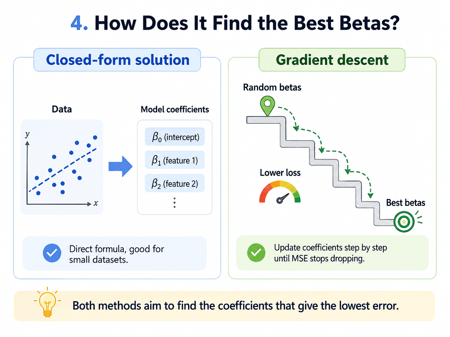
4. How Does It Actually Find the Best Betas?

Two ways.

• The closed-form solution. There is a one-shot formula (called the normal equation) that computes the optimal beta values directly. Fast for small datasets.
• Gradient descent. Start with random beta values, nudge them iteratively until MSE stops dropping. Necessary for big data, and the only realistic option once we move beyond linear regression to almost every other algorithm. We will dedicate [[Day 7 Gradient Descent — How Models Actually Learn|Day 7]] to it.

For now, we can trust that sklearn handles all of this for us.

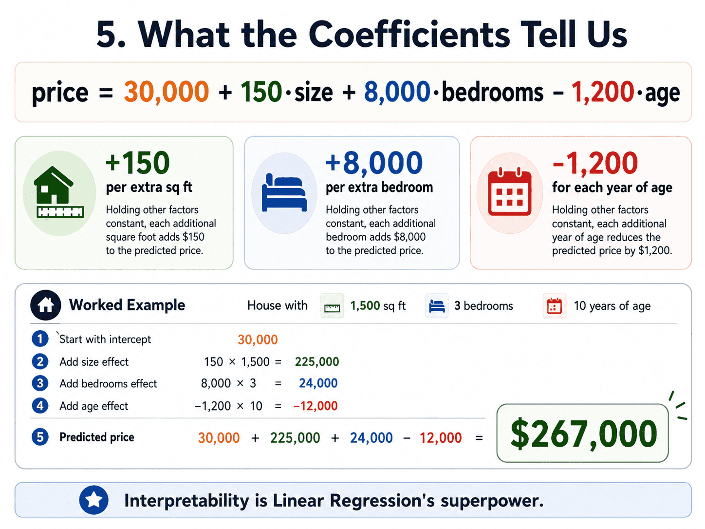
5. What the Coefficients Tell Us:

This is one of the biggest selling points of Linear Regression. The beta values are readable.

Say, after training on housing data, we get this model.

price = 30,000 + 150 · size + 8,000 · bedrooms − 1,200 · age

We can literally tell the business team that each extra square foot adds $150, each extra bedroom adds $8,000, and each year of age drops the price by $1,200. For a concrete prediction, plug in a 1,500 sq ft house with 3 bedrooms and 10 years of age: price = 30,000 + 150 × 1,500 + 8,000 × 3 + (−1,200) × 10 = 267,000. One model, one line, predictions on demand. Try doing that with a Random Forest. We cannot, easily. Interpretability is Linear Regression's superpower, and one of the main reasons it is still used in regulated industries like finance, insurance, and healthcare.

6. The Code:

from sklearn.linear_model import LinearRegression
from sklearn.model_selection import train_test_split

X_train, X_test, y_train, y_test = train_test_split(X, y, test_size=0.2)

model = LinearRegression()
model.fit(X_train, y_train)

print(model.coef_)         # the β₁, β₂, ...
print(model.intercept_)    # β₀
print(model.score(X_test, y_test))   # R² on the test set

The score method returns R² (R-squared), which is a score between 0 and 1 telling us how much of the variance in y our model explains. 1.0 is perfect, 0 is no better than always predicting the mean, and a negative R² means we are doing worse than that (yes, possible). We will properly meet R² and other evaluation metrics on Day 6 about Evaluation Metrics — How Do We Know a Model is Good.

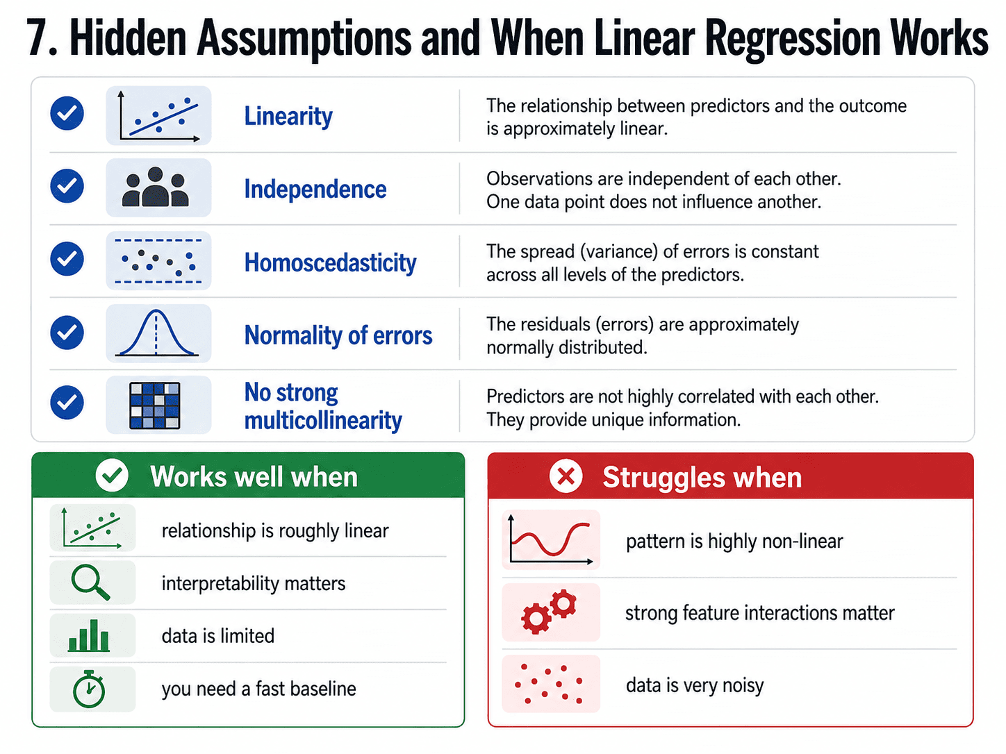
7. The Hidden Assumptions:

Linear Regression quietly assumes a few things. We do not need to memorise every one, but it is good to be aware.

• Linearity: The relationship between x and y is roughly a straight line.
• Independence: Rows do not influence each other.
• Homoscedasticity (fancy word, simple idea): The spread of errors is roughly constant across x values.
• Normality of errors: Errors are roughly bell-curved.
• No strong multicollinearity: Features should not be near-perfect copies of each other.

When these break badly, our coefficients become unreliable. In practice, mild violations are usually fine, and we only worry about the assumptions when interpreting the coefficients matters a lot (like in research or regulated industries).

8. When Linear Regression Wins, When It Loses:

It wins when the relationship really is roughly linear, when we need interpretability for stakeholders or audits, when we have limited data and fancier models would overfit, and when we need a fast lightweight baseline before reaching for anything heavier.

A small rule of thumb. Always try Linear Regression first. If a complex model cannot beat it by a meaningful margin, ship the linear one.

It loses when the pattern is highly non-linear (price doubling after a threshold), when there are strong feature interactions (effect of size depends on location), or when there is a lot of noise the linear model cannot soak up. For those, decision trees and ensembles (coming next week) handle the curvature naturally.

9. A Few Common Confusions Cleared:

• Why is it called "regression"? Historical baggage. Sir Francis Galton coined it when studying how children's heights "regressed toward the mean." The math stuck, and the name stuck.
• Why MSE and not just absolute error? Squared errors are smooth (differentiable), which makes the math and optimisation neat. Absolute error (MAE) is also valid and is more robust to outliers. Both are valid tools.
• Do I need to scale features for Linear Regression? Not strictly required for the math, but it is a good idea if features are on wildly different scales. It makes coefficients comparable and helps gradient descent converge faster.
• Is it always linear in the features? Not necessarily. We can feed it x² or log(x) as features. Then it is still linear in the coefficients but can curve in the input space.
• Most common interview gotcha? "If we double all the prices, what happens to the slope and intercept?" Both double. Easy to reason about, because the model is so transparent.

A small thought to sit with. If our Linear Regression has R² = 0.92 on training data but R² = 0.45 on test, recall [[Day 2 Train-Test Split & The Sin of Overfitting|Day 2]]'s table. That gap is variance, which means overfitting. With Linear Regression, overfitting usually means too many features relative to data. We could remove weak features, gather more rows, or apply regularisation, which is exactly what [[Day 9 Regularization — Ridge, Lasso, ElasticNet|Day 9]] will give us.

10. If This Came In An Interview:

A few questions to be ready for, with one-line answers.

• What is Linear Regression and what does it minimise? A model that draws a straight line through the data by minimising Mean Squared Error: the average of (actual − predicted)².
• What do the coefficients mean? Each one tells us how much the prediction changes per unit increase in that feature, holding the others constant.
• MSE vs MAE vs RMSE, when do you use which? MSE for math/optimisation. MAE when we want a metric robust to outliers. RMSE when we want MSE in the original units.
• What is R²? The fraction of variance in y the model explains. 1.0 is perfect, 0 means "no better than predicting the mean," negative means worse than that.
• What is multicollinearity and why does it matter? When features are highly correlated, coefficients become unstable and hard to interpret. The fix is to drop one, combine them, or use Ridge regularisation.
• Does Linear Regression need scaling? Not strictly for the math, but yes for fair regularisation and for comparing coefficients.

11. Summing It Up:

If we remember one thing from today, it is this: Linear Regression draws the line that makes the squared errors as small as possible. Each coefficient tells us how one feature shifts the prediction. Fragile for curvy data, brilliant as a baseline, and a stepping stone to almost every other algorithm in this series.

Coming Up on Day 5

Linear Regression predicts numbers. But what if the answer is yes or no, like "will this customer churn?" or "is this email spam?" Tomorrow, we meet the workhorse of classification, which is Logistic Regression. Despite the misleading name, it is a classification algorithm. We will see why, and we will meet the famous sigmoid curve.

That's all for today. Let's meet up again tomorrow with Day 5.

Thanks for reading.