Day 21: PCA — Shrinking Dimensions Without Losing Meaning

Three days of clustering grouped rows together. Today we tackle the opposite problem, which is too many columns. PCA is the most famous tool for shrinking high-dimensional data into a few directions that capture most of the meaning, and it shows up everywhere, from visualisation to preprocessing.

This blog post is a daily learning summary of my ML self-study.

Terms Used Today

Dimensionality reduction: Shrink the number of features while preserving most of the information.

Principal component (PC): A direction in feature space. PC1 captures the most variance, PC2 the second-most, and so on.

Explained variance ratio: The fraction of total spread each PC accounts for.

Orthogonal: Perpendicular. All PCs are perpendicular to each other.

Loadings: The weights showing how each original feature contributes to a PC.

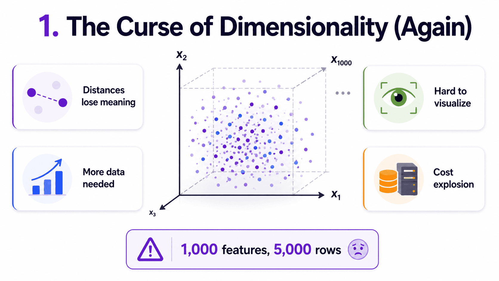
1. The Curse of Dimensionality (Again):

We brushed against this on Day 12 K-Nearest Neighbors — Tell Me Who Your Friends Are with KNN.

Today we face it head on.

In high dimensions, bad things happen.

Distances stop being informative (everything is "far" from everything).
Models need exponentially more data to train well.
Visualisation becomes impossible (humans live in 3D).
Storage and compute costs explode.

If we have 1,000 features but only 5,000 rows, our model is in trouble.

2. The Big Idea Behind PCA:

PCA stands for Principal Component Analysis.

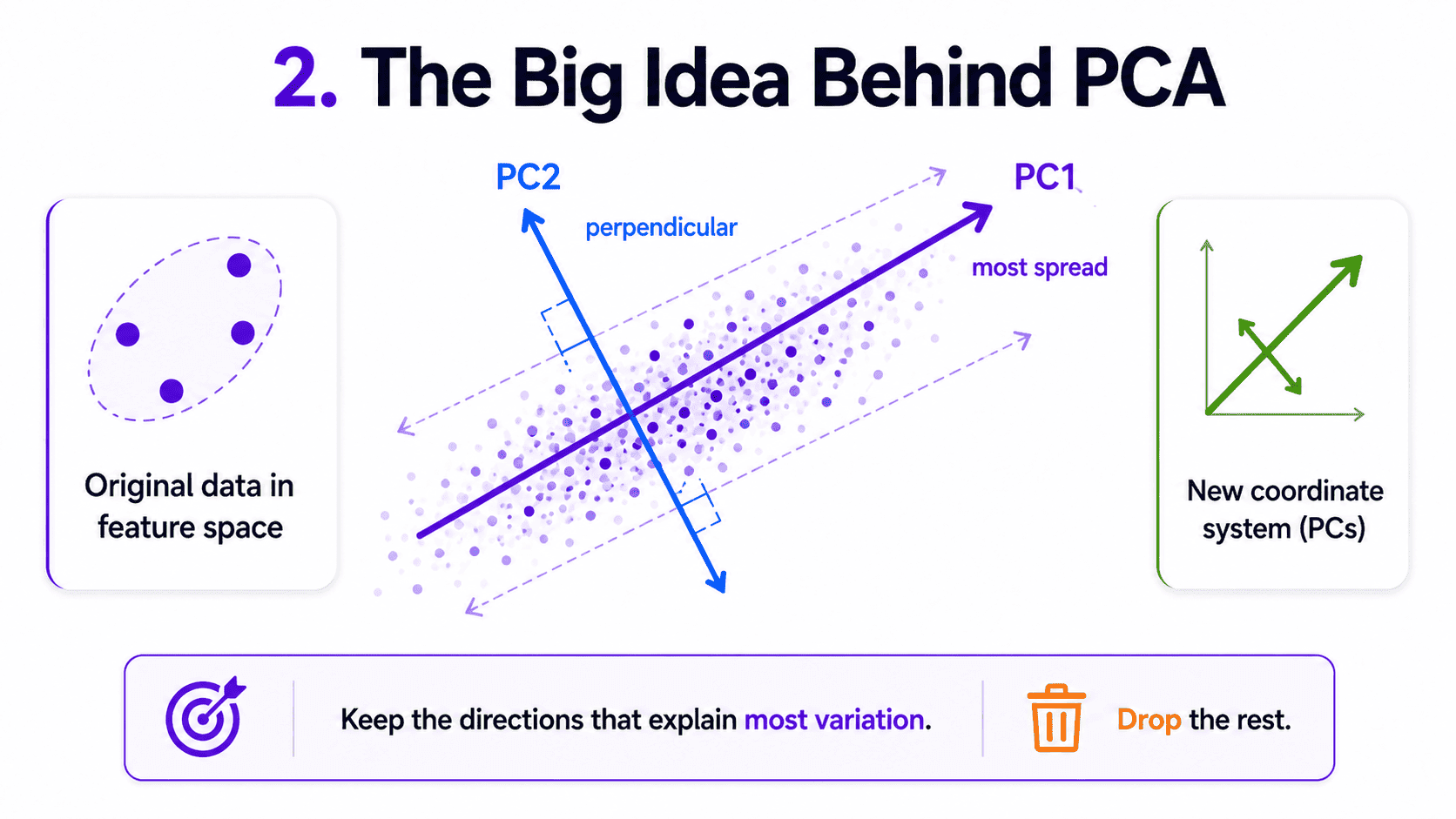
Imagine our data is a cloud of points in 100-dimensional space. PCA asks:

"Which direction in this cloud has the most spread?"

That direction is Principal Component 1 (PC1). Then it asks:

"Which direction, perpendicular to PC1, has the most spread?"

That is PC2. Repeat for PC3, PC4, and so on.

We end up with a new coordinate system, aligned with the directions of largest variation in our data. The cool part is that we can usually throw away most of the new dimensions, because they have almost no variation, and lose very little information.

PCA finds the few directions that explain most of the data, then drops the rest.

3. A Simple Picture:

Suppose our data lives roughly along a diagonal line in 2D. 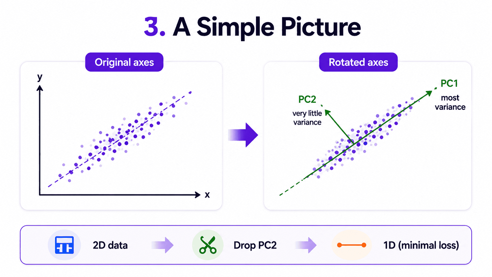We could describe each point with (x, y) coordinates. But almost all the variation is along the diagonal. The perpendicular direction is barely used.

PCA rotates the axes so PC1 points along the diagonal and PC2 sits perpendicular to it. Now PC1 captures roughly 95% of the variance. We drop PC2 and we have gone from 2D to 1D with almost no loss.

In a 100-dimensional dataset, this can be 100 dimensions reduced to 10 with minimal information loss. That is the magic.

4. Explained Variance:

After PCA, each principal component has an explained variance ratio, which is the fraction of total spread it accounts for. 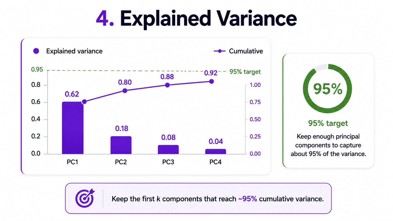Cumulatively, PC1 plus PC2 explain 0.80 of the spread. So the first two components capture 80% of the data's variation. A common rule of thumb is to keep enough PCs to capture 95% of the variance (or 90%, or 80%, depending on the use case).

from sklearn.decomposition import PCA
pca = PCA(n_components=0.95)   # keep enough to explain 95% variance
X_pca = pca.fit_transform(X_scaled)
print(X_pca.shape)

This automatically picks the right number of components for us. Clean and elegant.

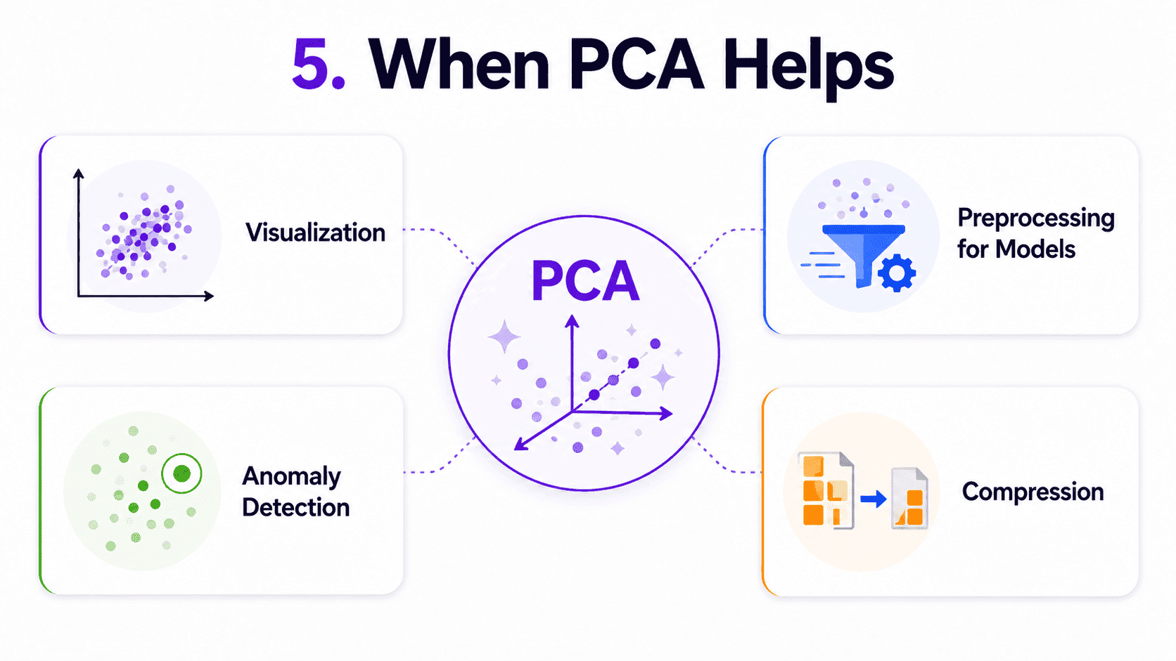
5. When PCA Helps:

Visualisation. Reduce to 2 or 3 components and plot. Even a 100-dim dataset can show clusters and structure when projected to 2D.

Preprocessing for other models.

Noise reduction: drop weak components that are mostly noise.
Speed up training: fewer features mean faster everything.
Mitigate multicollinearity: PCA's components are uncorrelated by design.

Anomaly detection. If a point does not reconstruct well from the top components, it is an outlier.

Compression. Storing 50 components instead of 5,000 features saves space.

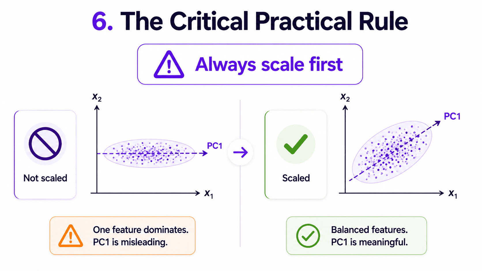
6. The Critical Practical Rule:

Always scale features before PCA.

PCA is driven by variance. Features on large scales (income in dollars) will dominate PC1 entirely, drowning out smaller-scale features (age in years).

from sklearn.preprocessing import StandardScaler
from sklearn.decomposition import PCA

X_scaled = StandardScaler().fit_transform(X)
pca = PCA(n_components=10)
X_reduced = pca.fit_transform(X_scaled)

This is the most common PCA bug in beginner code.

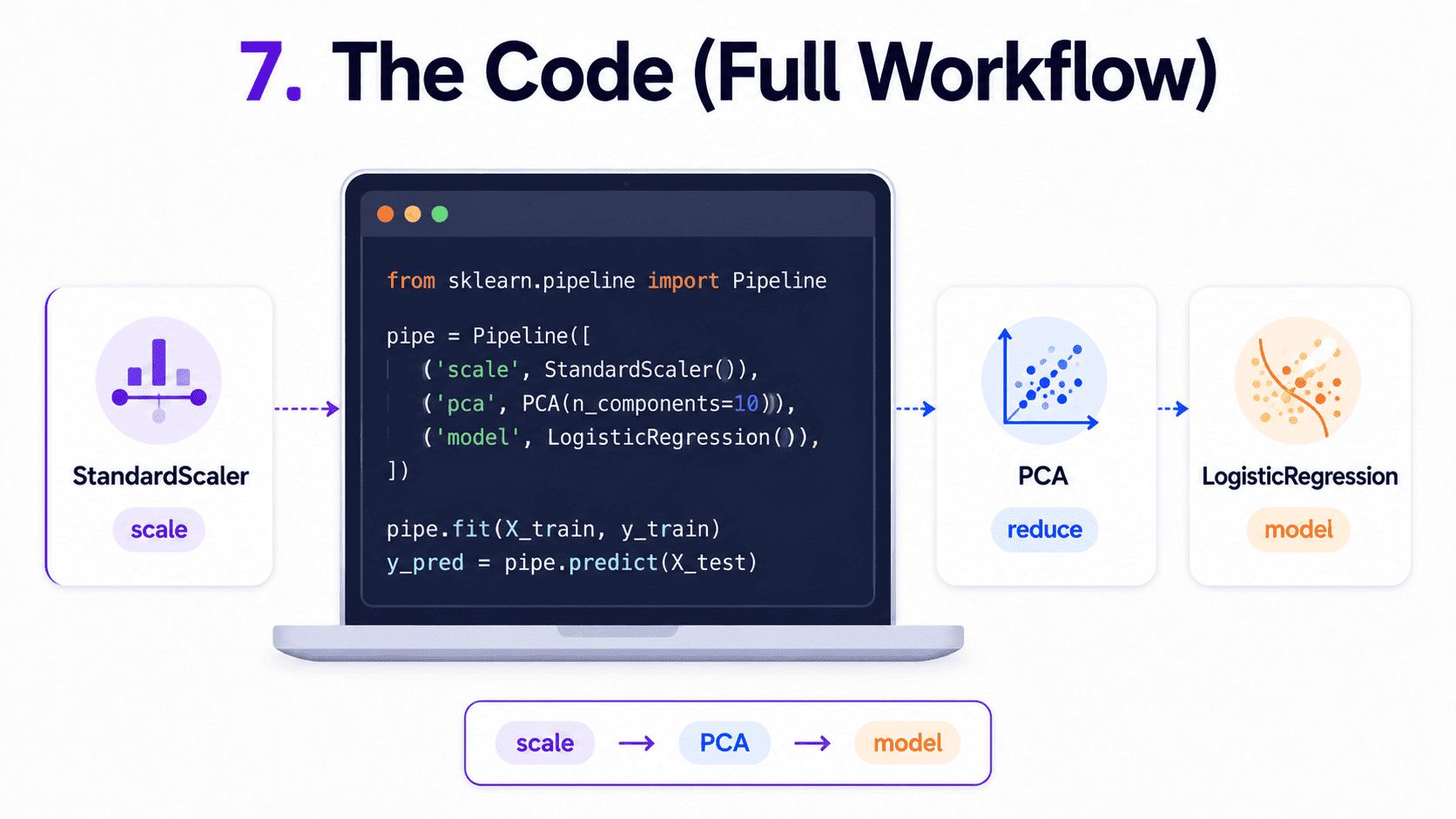
7. The Code (Full Workflow):

from sklearn.preprocessing import StandardScaler
from sklearn.decomposition import PCA
from sklearn.pipeline import Pipeline
from sklearn.linear_model import LogisticRegression

pipe = Pipeline([
    ('scaler', StandardScaler()),
    ('pca', PCA(n_components=0.95)),
    ('clf', LogisticRegression(max_iter=1000))
])
pipe.fit(X_train, y_train)
print("Test score:", pipe.score(X_test, y_test))

# Inspect what PCA kept
pca = pipe.named_steps['pca']
print("Components kept:", pca.n_components_)
print("Variance explained per PC:", pca.explained_variance_ratio_[:5])

The standard pipeline pattern: scale, PCA, model. It cleanly handles training and inference.

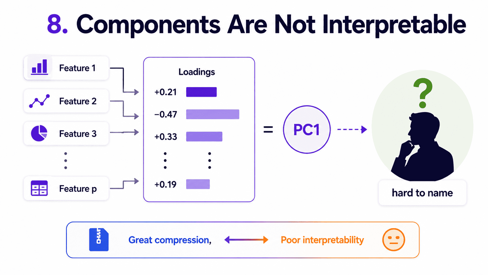
8. Components Are Not Interpretable:

PC1 is a combination of all the original features. We can inspect the weights.

import pandas as pd
loadings = pd.DataFrame(pca.components_[:3], columns=feature_names)

But "0.42 × income − 0.31 × age + 0.18 × tenure ..." is rarely something we can name in business terms. PCA trades interpretability for compression. We should be honest about this trade.

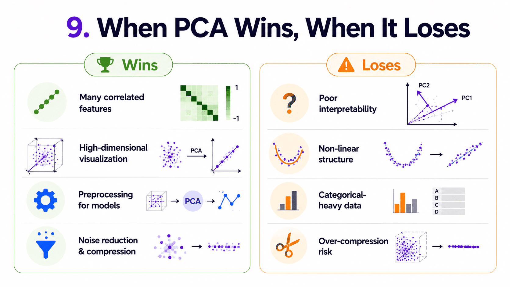
9. When PCA Wins, When It Loses:

It wins on many correlated features (sensor data, image pixels, gene expressions). When we need to visualise high-dim data in 2D or 3D. When we are preprocessing for an algorithm that struggles in high dim (Day 12 K-Nearest Neighbors — Tell Me Who Your Friends Are, Day 18 Unsupervised Learning & K-Means — Finding Hidden Groups). And when we suspect most features are noise.

It loses when categorical features dominate (PCA needs continuous, scaled inputs). When important info is non-linear (use t-SNE or UMAP for visualisation, autoencoders for ML).

When interpretability is critical (combinations of features are hard to explain). And when we have few features to begin with, since PCA pays off when there are many redundant features.

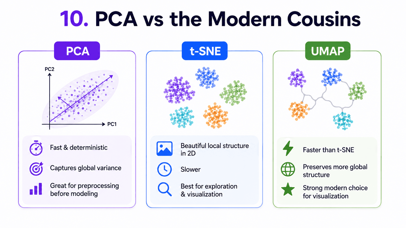
10. PCA vs the Modern Cousins (Just to Be Aware):

For visualisation specifically:

t-SNE: preserves local structure beautifully. Slow. Famous for 2D plots.
UMAP: like t-SNE but faster. Preserves more global structure. The newer favourite.

Both are non-linear and beat PCA at 2D visualisation. But they are not great for general dimensionality reduction before modelling. PCA still wins there because it is fast, deterministic, and invertible.

A small thought to sit with. Suppose our dataset has 2,000 columns and only 1,500 rows. Random Forest is overfitting badly.

Should we reach for PCA?

Maybe. PCA could shrink to say 50 components capturing 95% of variance, leaving Random Forest much better behaved. But we should also consider other angles.

Feature selection could pick the top features by importance, with no transformation needed and keeping interpretability. Regularised linear models like Lasso can effectively drop irrelevant features for free. And more data, if possible, is the simplest fix.

PCA is one tool, not the only tool. Often Lasso or feature importance does the same job more transparently.

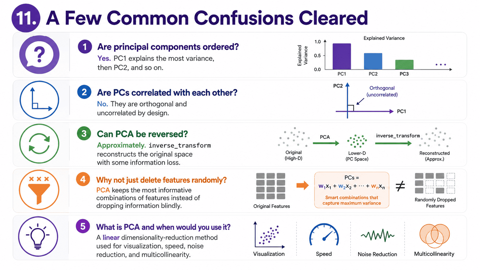
11. A Few Common Confusions Cleared:

Are principal components ordered? Yes, by decreasing explained variance. PC1 explains the most, PC2 the next, and so on.
Are PCs correlated with each other? No. They are orthogonal (perpendicular) by construction. This is also why PCA is useful for fixing multicollinearity in linear models.
Can PCA be reversed? Yes (approximately). pca.inverse_transform(X_pca) reconstructs the original space, with some loss equal to the variance we dropped.
Why not just delete features randomly? Because each feature carries some unique information. PCA combines features so the kept directions are the most informative combinations.
Common interview question: "What is PCA and when would you use it?" A linear dimensionality reduction that finds the directions of maximum variance and projects data onto the top few. We use it for visualisation, speed, noise reduction, and dealing with multicollinearity. Always scale features first. Components are not interpretable.

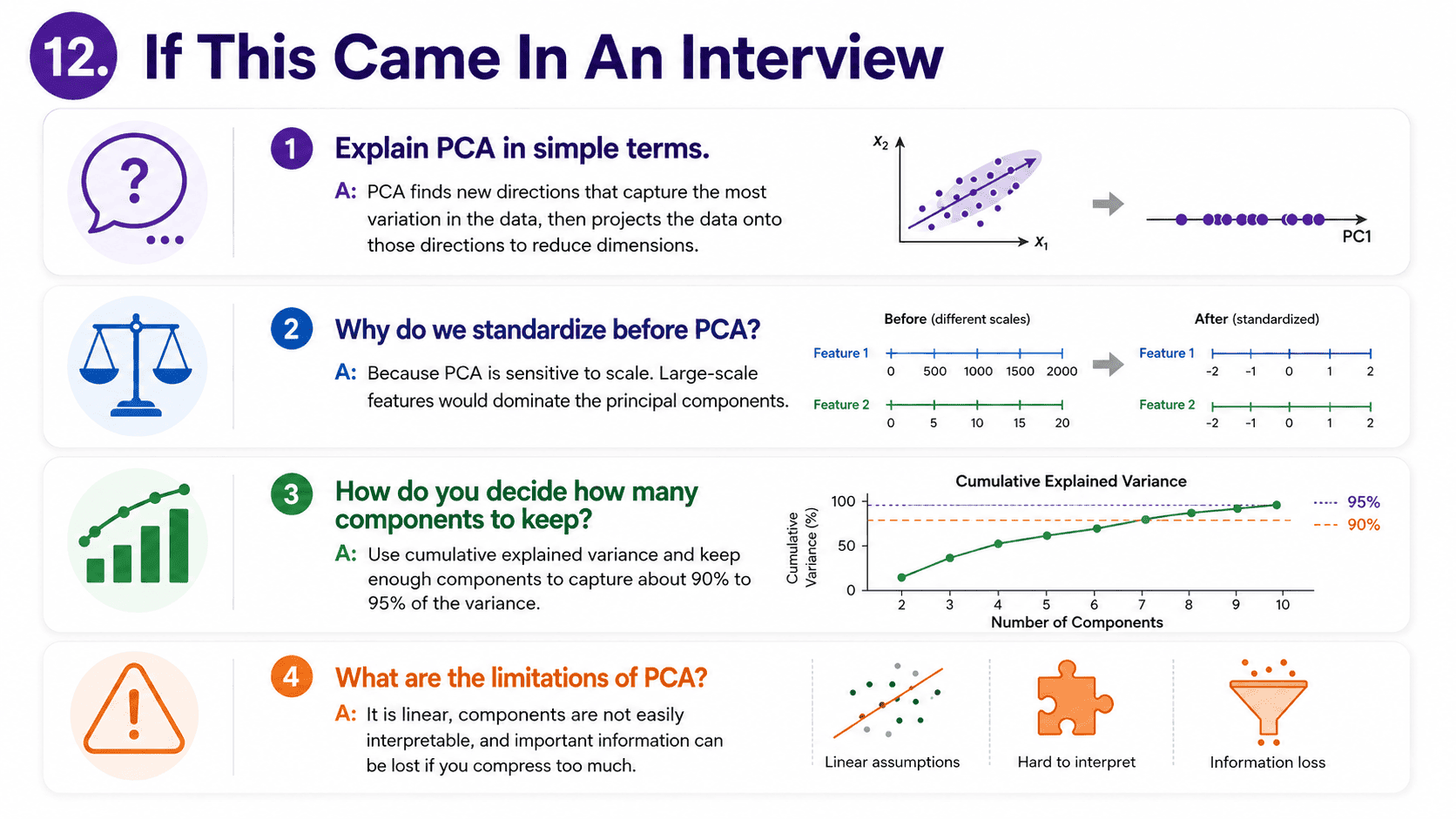
12. If This Came In An Interview:

A few questions to be ready for, with one-line answers.

What is PCA? A linear dimensionality reduction that finds the directions of maximum variance in the data, then projects everything onto the top few.
When would you use PCA? For visualisation in 2D or 3D, to speed up training, to reduce noise, to mitigate multicollinearity, or as preprocessing for algorithms that struggle in high dimensions (KNN, K-Means).
Why must you scale features first? PCA is driven by variance. Features on bigger scales would dominate PC1 unfairly. Always StandardScale before PCA.
Are principal components interpretable? No. Each PC is a combination of all original features. We can inspect the loadings, but rarely give the components a clean business name.
What is the explained variance ratio? The fraction of total variance each principal component accounts for. We pick K by keeping enough components to hit (say) 95% of cumulative variance.
PCA vs feature selection? PCA combines features into new directions. Feature selection picks a subset of original features. PCA gives a tighter representation, feature selection keeps interpretability.
PCA vs t-SNE / UMAP? PCA is linear, fast, and deterministic, so better for general dimensionality reduction. t-SNE and UMAP are non-linear and better for 2D visualisation, but slower and not invertible.

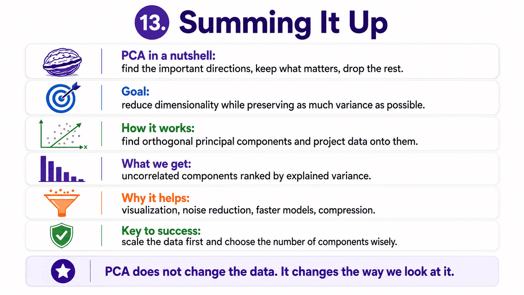
13. Summing It Up:

If we remember one thing from today, it is this: PCA finds the few directions that explain most of the data, and throws the rest away. Always scale features first. Choose K via cumulative explained variance (95% is a common target). Fast, deterministic, and a great preprocessing step, but the components are not human-interpretable.

Coming Up on Day 22 Data Leakage, ML Workflow & Interview Cheat Sheet

This is the final stretch. Tomorrow we tie everything together with the practical, end-to-end ML workflow, the silent killer that breaks pipelines (data leakage), and an interview cheat sheet covering every "why" question we have raised in twenty-one days.

That's all for today. Let's meet up again tomorrow with Day 22.

Thanks for reading.

Cheers!