Day 20: DBSCAN — Clusters by Density Not Distance

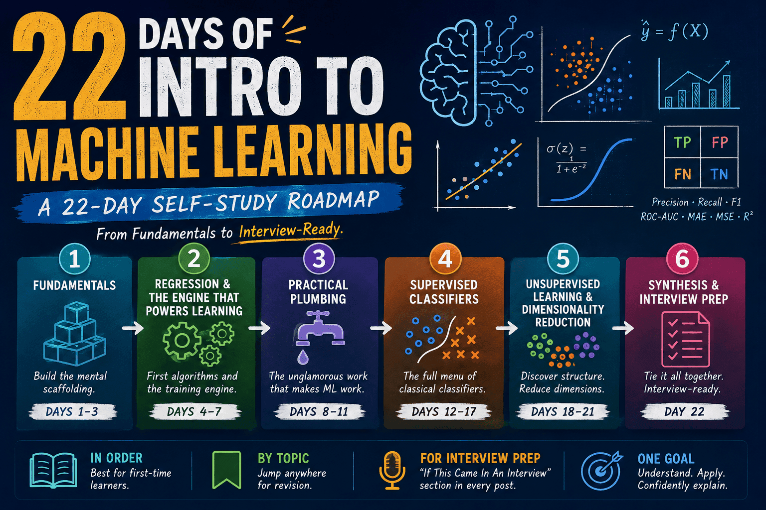
K-Means and Hierarchical clustering both assume our groups are roughly globular. But what about ring-shaped clusters? Crescent moons? Data scattered with random outliers?

DBSCAN handles all of them, and on top of that, it does not require us to know K in advance.

This blog post is a daily learning summary of my ML self-study.

Terms Used Today

• Density-based clustering: Define a cluster as a dense region of points.
• Core point: A point with at least min_samples neighbours within radius eps.
• Border point: A point close enough to a core point but not a core itself.
• Noise point: A point that is neither core nor border. Gets label -1 in sklearn.
• eps (ε): The neighbourhood radius.
• min_samples: The minimum density to be a core point.

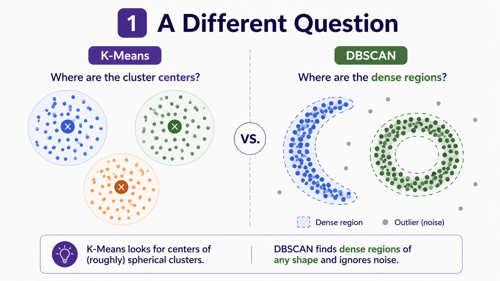
1. A Different Question:

Day 18: Unsupervised Learning & K-Means — Finding Hidden Groups asked "Where are the cluster centres?". DBSCAN asks "Where are the dense regions?".

A cluster is just a connected blob of densely-packed points. Whatever shape that blob makes (circle, banana, snake), DBSCAN finds it. DBSCAN stands for Density-Based Spatial Clustering of Applications with Noise.

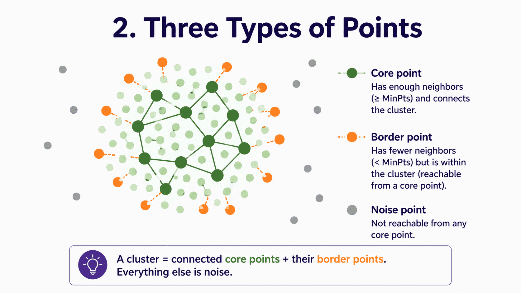
2. Three Types of Points:

DBSCAN labels every point as one of three kinds.

• Core point. Has many neighbours within a small radius. The heart of a cluster.
• Border point. Sits near a core point but does not have enough neighbours itself to be a core.
• Noise point. Alone in empty space. Does not belong to any cluster.

A cluster is then all core points connected to each other, plus their border points. Everything else is noise.

DBSCAN does not force every point into a cluster. Some points are simply labelled "noise."

This is a huge advantage in real-world data full of weirdos.

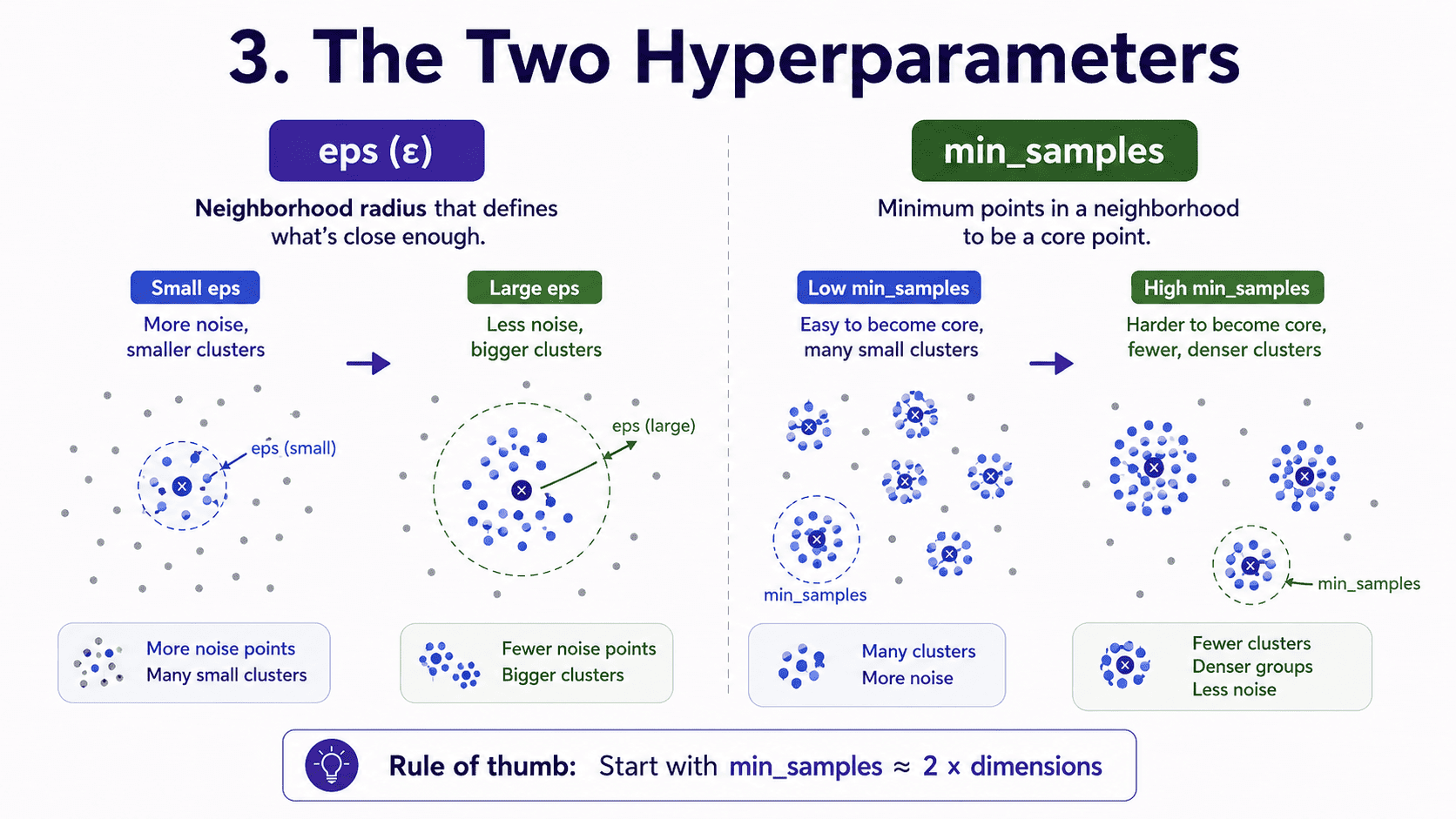
3. The Two Hyperparameters:

eps (ε): the radius around each point that defines its "neighbourhood."

• Small eps → fewer points are considered close → smaller clusters, more noise.
• Large eps → many points are considered close → bigger clusters, less noise.

min_samples: the minimum number of points within eps to count as a core point.

• Small min_samples → easy to be a core → many small clusters.
• Large min_samples → harder to be a core → fewer, denser clusters.

Rule of thumb. min_samples ≈ 2 × number of dimensions. For 2D data, start with 4 or 5.

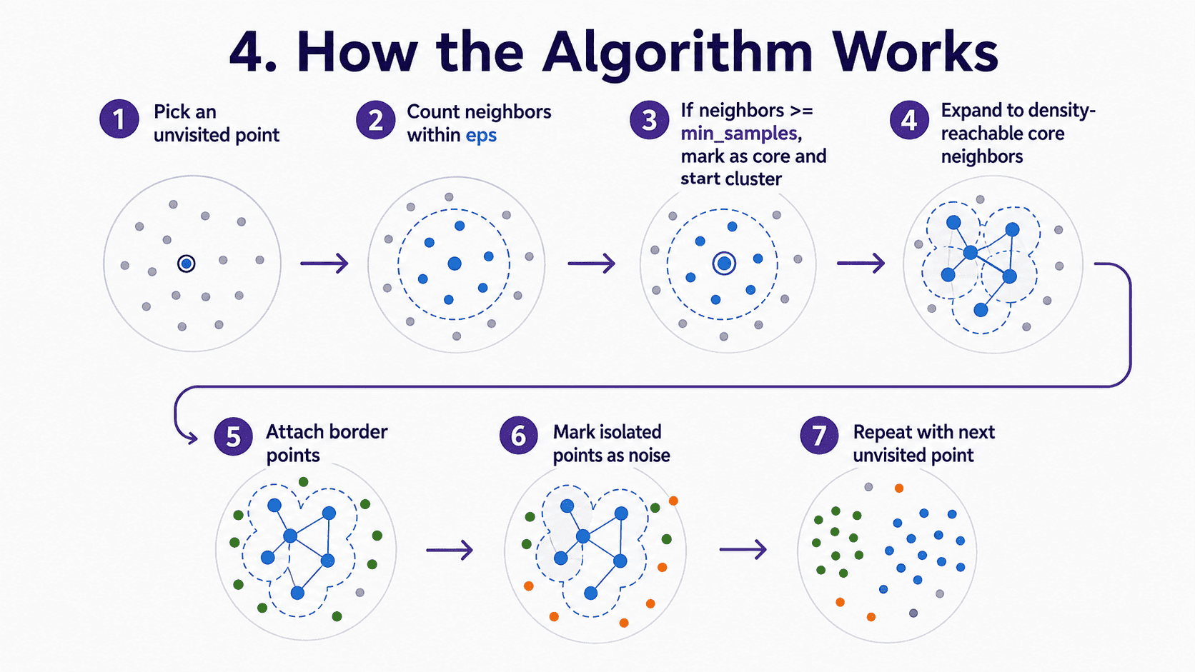
4. How the Algorithm Works:

1. Pick any unvisited point.
2. Count its neighbours within eps.
3. If neighbours ≥ min_samples, it is a core point. Start a new cluster.
4. Recursively absorb all density-reachable points (their neighbours, and their neighbours' neighbours, if those are also cores).
5. Border points (close to a core but not a core themselves) join the cluster.
6. Points without enough neighbours and not adjacent to any core are labelled as noise.
7. Move to the next unvisited point. Repeat.

The result is as many clusters as the density structure naturally has. No K to choose.

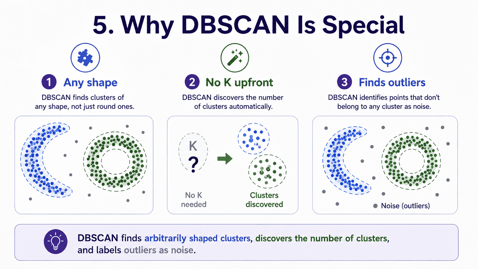
5. Why DBSCAN Is Special:

Three properties make it stand out.

• Finds arbitrarily shaped clusters: rings, spirals, crescents, anything connected.
• Does not need K upfront: the algorithm discovers how many clusters exist.
• Identifies outliers natively: noise points are clusters' leftovers.

Show DBSCAN the classic "two crescent moons" dataset that breaks K-Means, and it nails it.

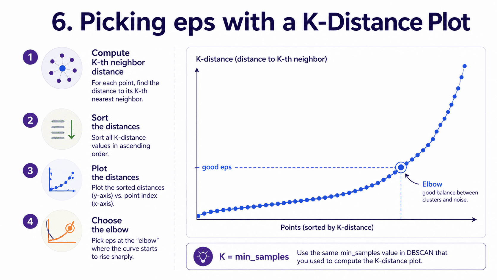
6. Picking eps with a K-Distance Plot:

eps is the trickiest hyperparameter. A common heuristic.

1. For each point, find the distance to its K-th nearest neighbour (K = min_samples).
2. Sort those distances in increasing order.
3. Plot them.
4. Look for an elbow. The y value at the elbow is a good eps.

from sklearn.neighbors import NearestNeighbors
import numpy as np
import matplotlib.pyplot as plt

nbrs = NearestNeighbors(n_neighbors=5).fit(X_scaled)
distances, _ = nbrs.kneighbors(X_scaled)
distances = np.sort(distances[:, -1])
plt.plot(distances)
plt.show()

Similar in spirit to the Day 18: Unsupervised Learning & K-Means — Finding Hidden Groups, applied to the right knob.

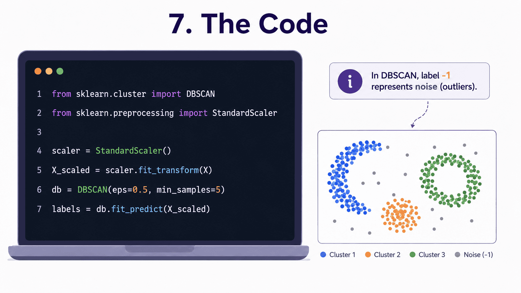
7. The Code:

from sklearn.cluster import DBSCAN
from sklearn.preprocessing import StandardScaler

X_scaled = StandardScaler().fit_transform(X)

db = DBSCAN(eps=0.5, min_samples=5)
labels = db.fit_predict(X_scaled)

print("Clusters found:", len(set(labels)) - (1 if -1 in labels else 0))
print("Noise points:", (labels == -1).sum())

A cluster label of -1 always means noise in DBSCAN. Everything else is cluster 0, 1, 2, and so on.

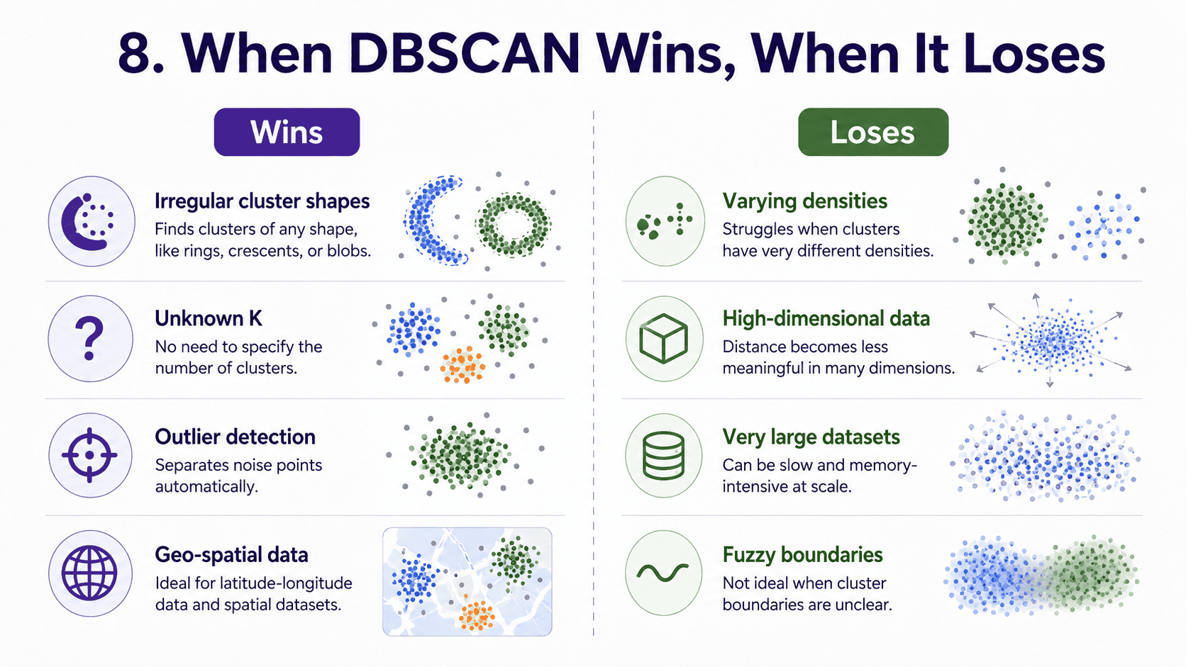
8. When DBSCAN Wins, When It Loses:

It wins when cluster shapes are irregular. When we do not know how many clusters exist. When data has outliers we want flagged. When density varies enough to define structure. Geo data is a perfect fit, since geographic clusters often have arbitrary shapes.

It loses when clusters have varying density, since one eps cannot serve dense and sparse clusters equally. Use HDBSCAN (an extension) for this. On high dimensions, the curse of dimensionality strikes and "density" becomes meaningless.

On big datasets, naive DBSCAN is O(N²). sklearn uses tree-based indexing to speed this up, but it still struggles past a few hundred thousand rows. And when cluster boundaries are fuzzy, DBSCAN's hard density threshold does not degrade gracefully.

9. DBSCAN vs K-Means vs Hierarchical:

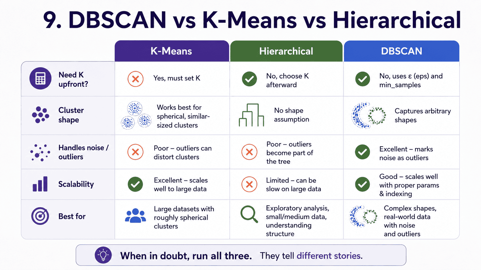
The clustering trio. When in doubt, run all three. They tell different stories about the same data.

A small thought to sit with.

Suppose we are clustering credit card transactions to find fraud rings. Most of our data is normal. A small percentage are weird, scattered, individual cases (one-off fraud). And a few clusters of suspicious patterns are real fraud rings.

Which algorithm fits this?

DBSCAN. We do not know K. Fraud rings have arbitrary shapes (groups of transactions sharing odd patterns). And we actively want outliers flagged as noise, since those individual weird transactions are interesting too.

K-Means would force every transaction into one of K clusters, hiding the outliers.

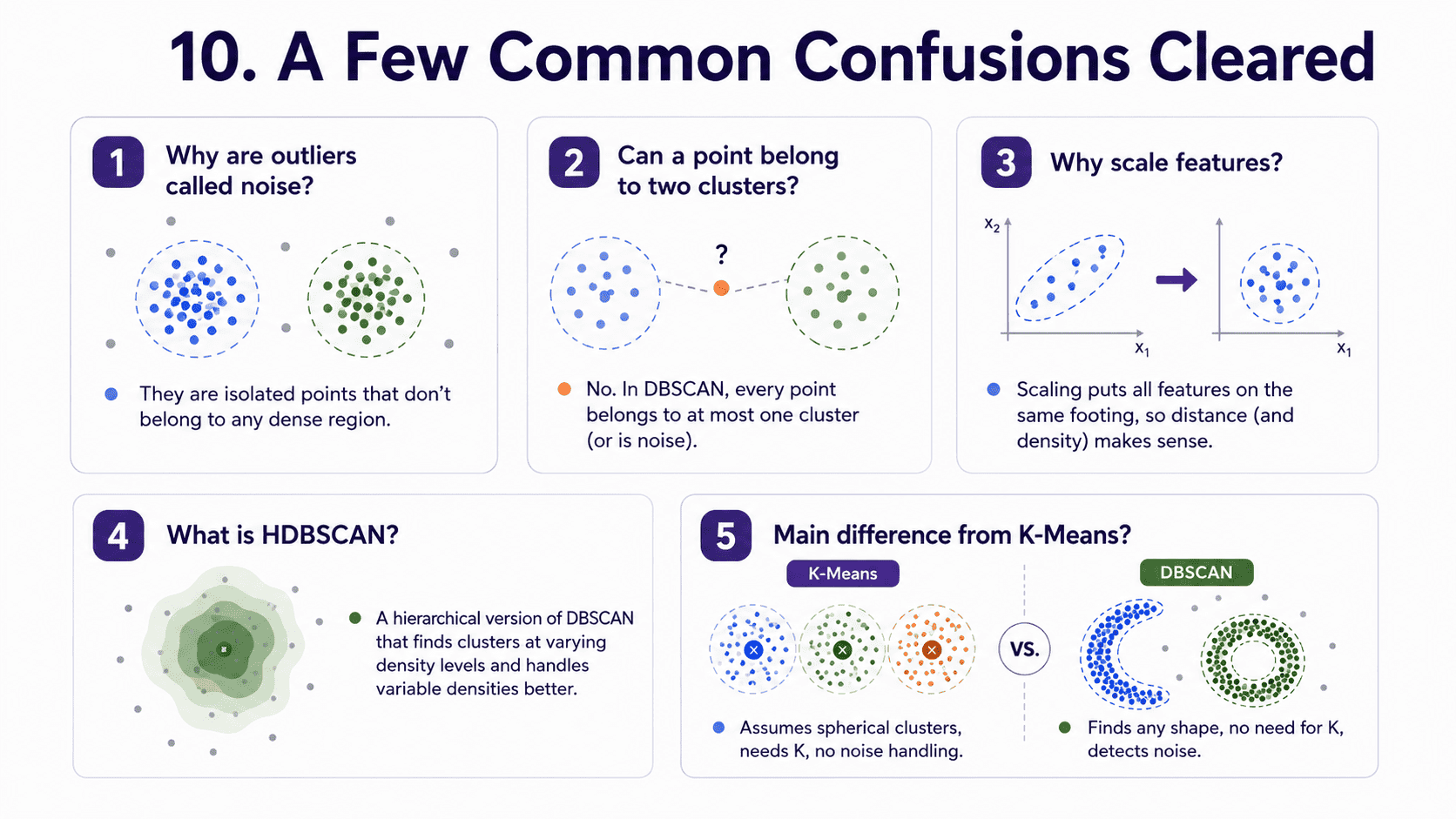
10. A Few Common Confusions Cleared:

• Why does DBSCAN call outliers "noise"? Because they are left over after the density structure has been discovered. They are not "wrong"; they are just not part of any dense cluster.
• Can a point belong to two clusters? No. Assignments are exclusive. If a point is border-reachable to two clusters' cores, sklearn assigns it to whichever it visits first (slight non-determinism).
• Why scale features? DBSCAN uses distances. Yes, scaling matters here too. Use StandardScaler.
• What is HDBSCAN? A modern extension that handles varying densities by automatically choosing different eps for different regions. Often a better default than DBSCAN. Worth knowing the name.
• Common interview question: "What is the main difference between K-Means and DBSCAN?" K-Means partitions every point into exactly one of K spherical clusters and requires K upfront. DBSCAN finds dense regions of arbitrary shape, discovers the number of clusters automatically, and labels low-density points as noise.

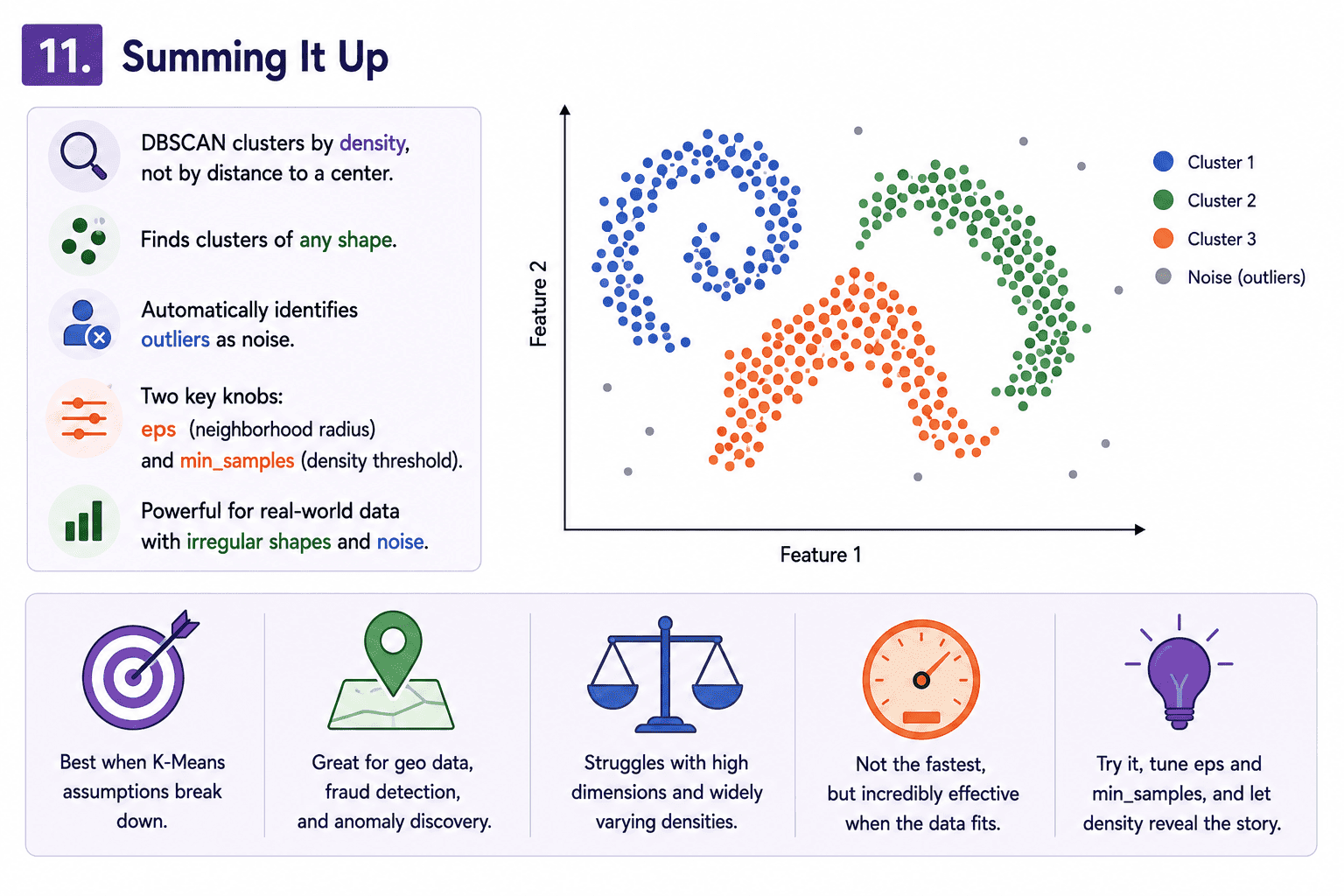
11. Summing It Up:

If we remember one thing from today, it is this: DBSCAN clusters by density, finds any shape, and labels outliers as noise. The two knobs are eps (neighbourhood radius) and min_samples (density threshold). Beautiful when K-Means' spherical assumption breaks down. Struggles in high dimensions and with widely varying cluster densities.

Coming Up on Day 21 PCA — Shrinking Dimensions Without Losing Meaning

We have spent three days clustering rows. Tomorrow we tackle the complementary problem: too many columns. The curse of dimensionality, and the most famous solution to it, which is PCA. It is the single most useful tool for handling high-dimensional data.

That's all for today. Let's meet up again tomorrow with Day 21.

Thanks for reading.

Cheers!