Day 19: Hierarchical Clustering — A Family Tree for Data

K-Means demanded that we know K up front. Today's algorithm is the opposite. It builds a tree of every possible clustering, from "everything is one big cluster" to "every point is its own cluster," and lets us slice it wherever we want.

Welcome to Hierarchical Clustering.

This blog post is a daily learning summary of my ML self-study.

Terms Used Today

• Agglomerative: Bottom-up clustering. Start with each point alone and merge nearest pairs.
• Divisive: Top-down clustering. Start with everything together and split recursively.
• Dendrogram: The tree picture showing every merge. We cut it horizontally to choose K.
• Linkage: How we measure "distance between two clusters" (single, complete, average, Ward).
• Ward linkage: sklearn's default. Merges to minimise the increase in total variance.

1. A Family Tree of Data:

Picture biologists organising species. 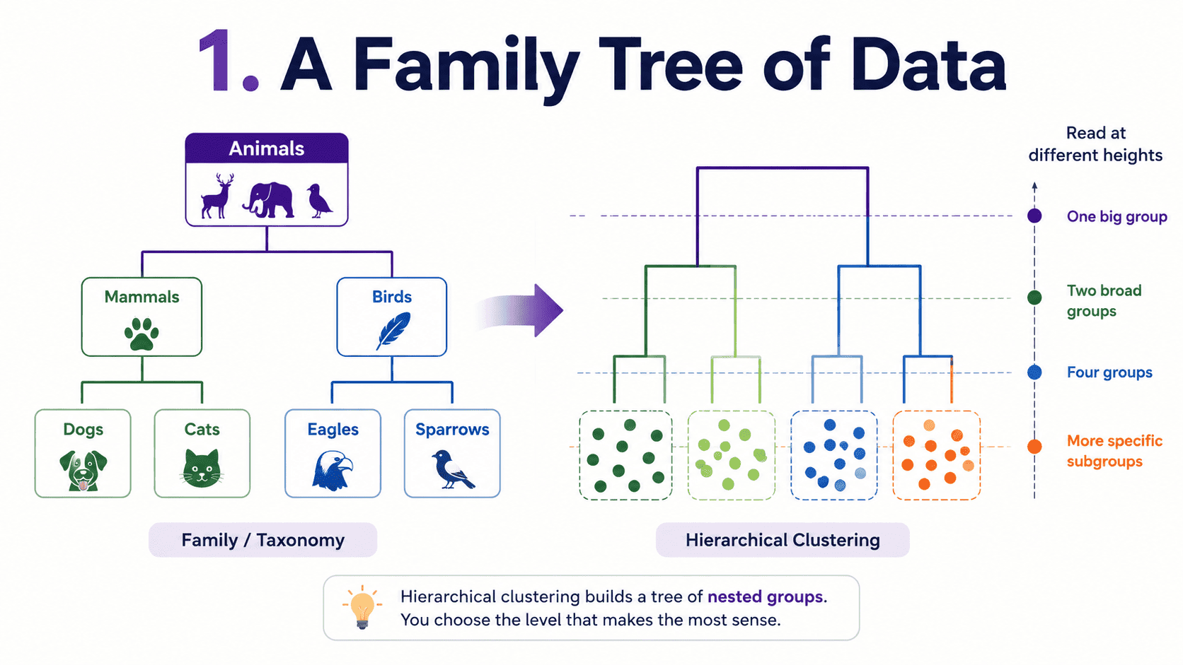Each level groups similar things. Cousins sit close, and distant relatives sit further apart. We can read groupings at any height, broad ("Animals") or specific ("Dogs"). Hierarchical clustering does the same thing for data. It builds a tree (called a dendrogram) showing how everything relates.

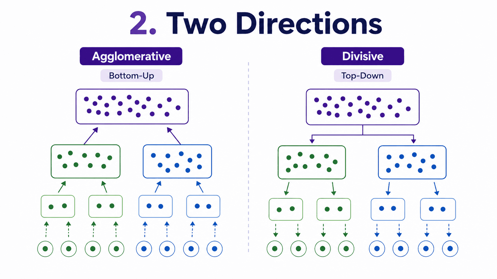
2. Two Directions:

Agglomerative (Bottom-Up). Start with every point in its own cluster (N clusters for N points). Then:

1. Find the two closest clusters.
2. Merge them into one.
3. Repeat until everything is in one cluster.

We build the tree upward, fusing as we go. This is the common version, and it is what sklearn implements.

Divisive (Top-Down). Start with everything in one cluster. Then:

1. Split it into two.
2. Recursively split each piece.

Mathematically clean, but rarely used in practice. We focus on agglomerative for the rest of this post.

3. The Dendrogram:

The output is not a fixed number of clusters. It is a tree showing the entire merging history. 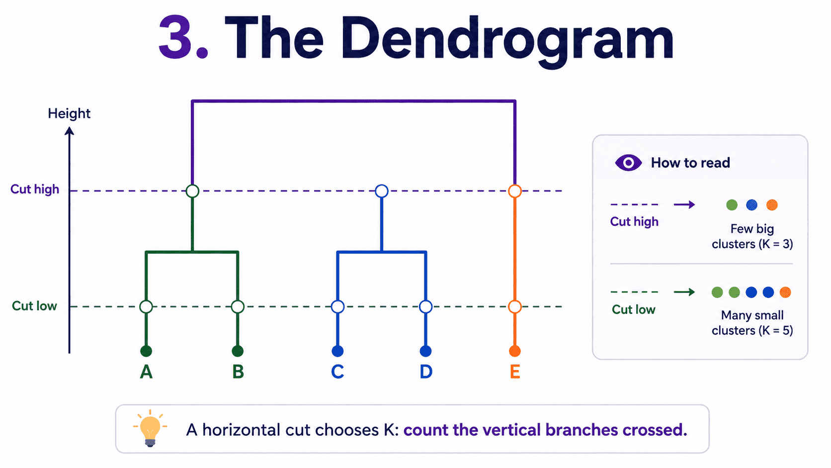To get K clusters, we draw a horizontal line at some height. The number of vertical lines we cross is K. This makes choosing K interactive.

• Cut high → few big clusters.
• Cut low → many small clusters.

The dendrogram is one of the most informative pictures in ML, and stakeholders love it.

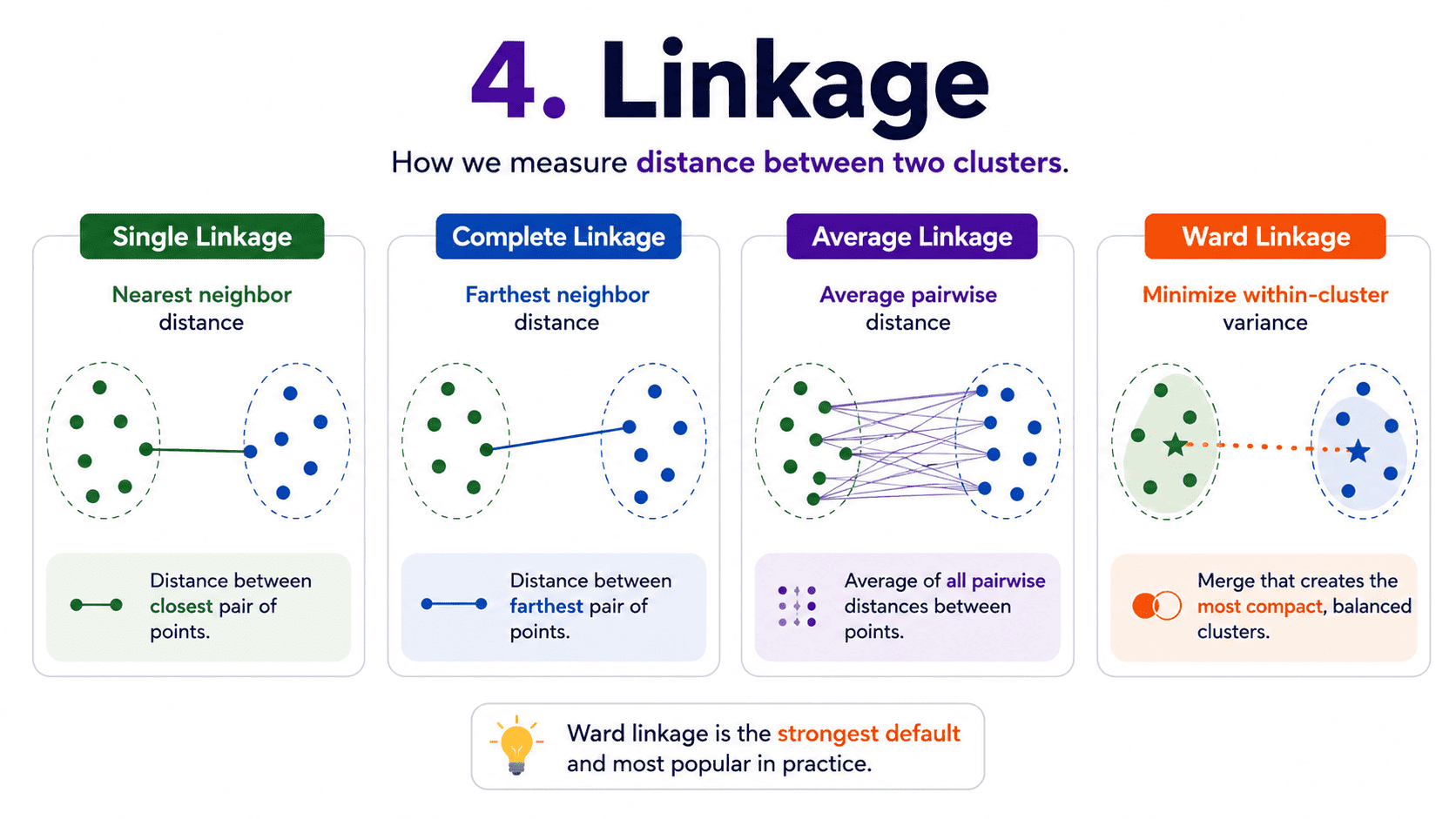
4. Linkage:

When two clusters each contain multiple points, how do we measure their distance? Five common choices, called linkage methods.

Single Linkage. Distance equals the closest pair across the two clusters.

• Can produce long stringy clusters ("chaining").
• Sensitive to noise.

Complete Linkage. Distance equals the farthest pair across the two clusters.

• Produces compact, similar-sized clusters.
• Sensitive to outliers.

Average Linkage. Distance equals the average of all pairwise distances between the clusters.

• Middle-of-the-road choice. Reasonable default.

Ward Linkage (Most Popular). Merges the two clusters that result in the smallest increase in total variance, similar in spirit to K-Means.

• Produces compact, balanced clusters.
• This is the sklearn default, and a strong baseline.

Centroid Linkage. Distance between cluster centroids. Less commonly used.

The practical advice is to default to Ward linkage unless we have a specific reason otherwise.

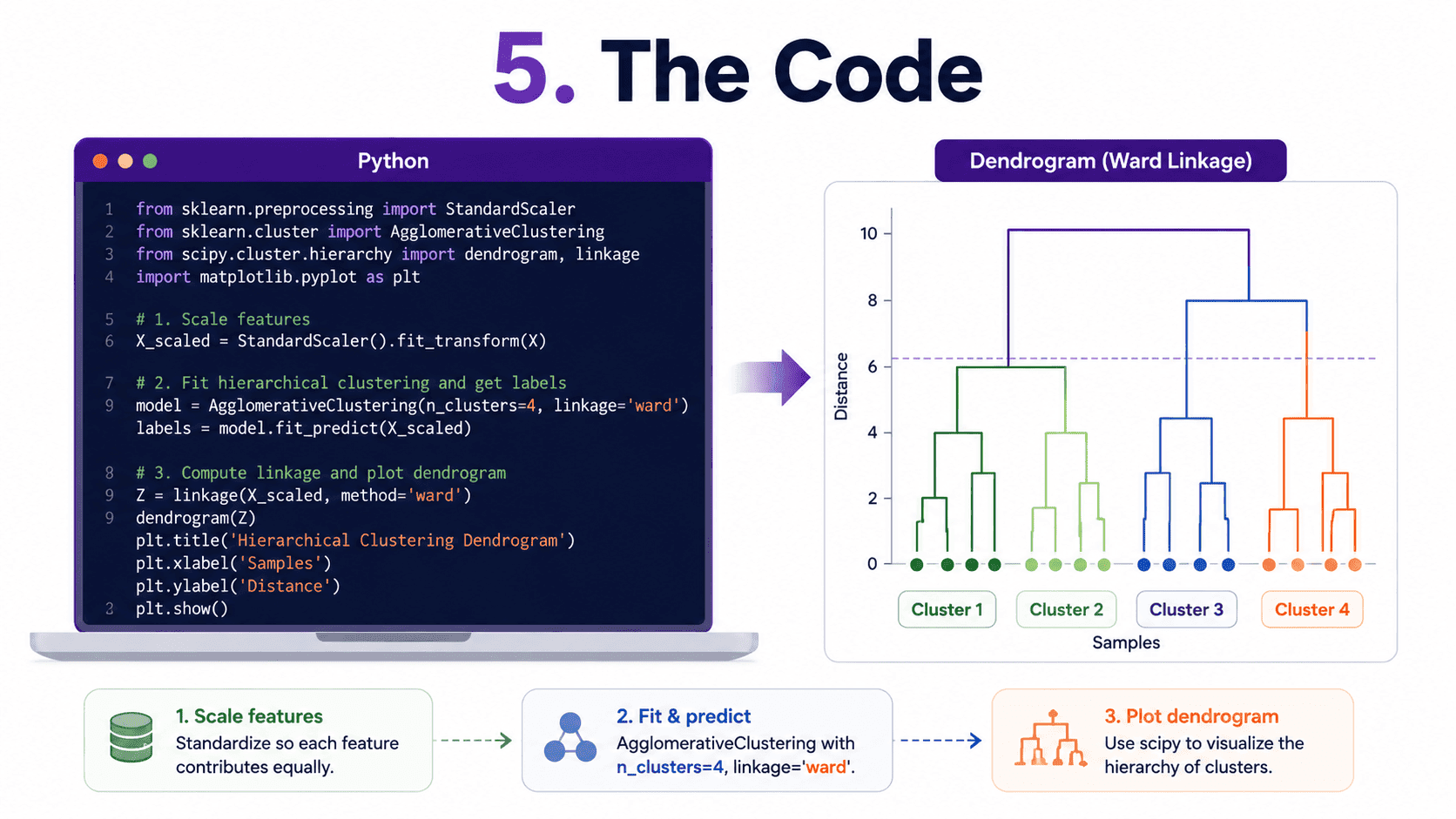
5. The Code:

from sklearn.cluster import AgglomerativeClustering
from sklearn.preprocessing import StandardScaler
import numpy as np

X_scaled = StandardScaler().fit_transform(X)

model = AgglomerativeClustering(n_clusters=4, linkage='ward')
labels = model.fit_predict(X_scaled)

For the dendrogram itself, we use scipy.

from scipy.cluster.hierarchy import linkage, dendrogram
import matplotlib.pyplot as plt

Z = linkage(X_scaled, method='ward')
dendrogram(Z, truncate_mode='lastp', p=30)
plt.show()

This gives us the picture. Always plot the dendrogram first. It is worth a thousand silhouette scores.

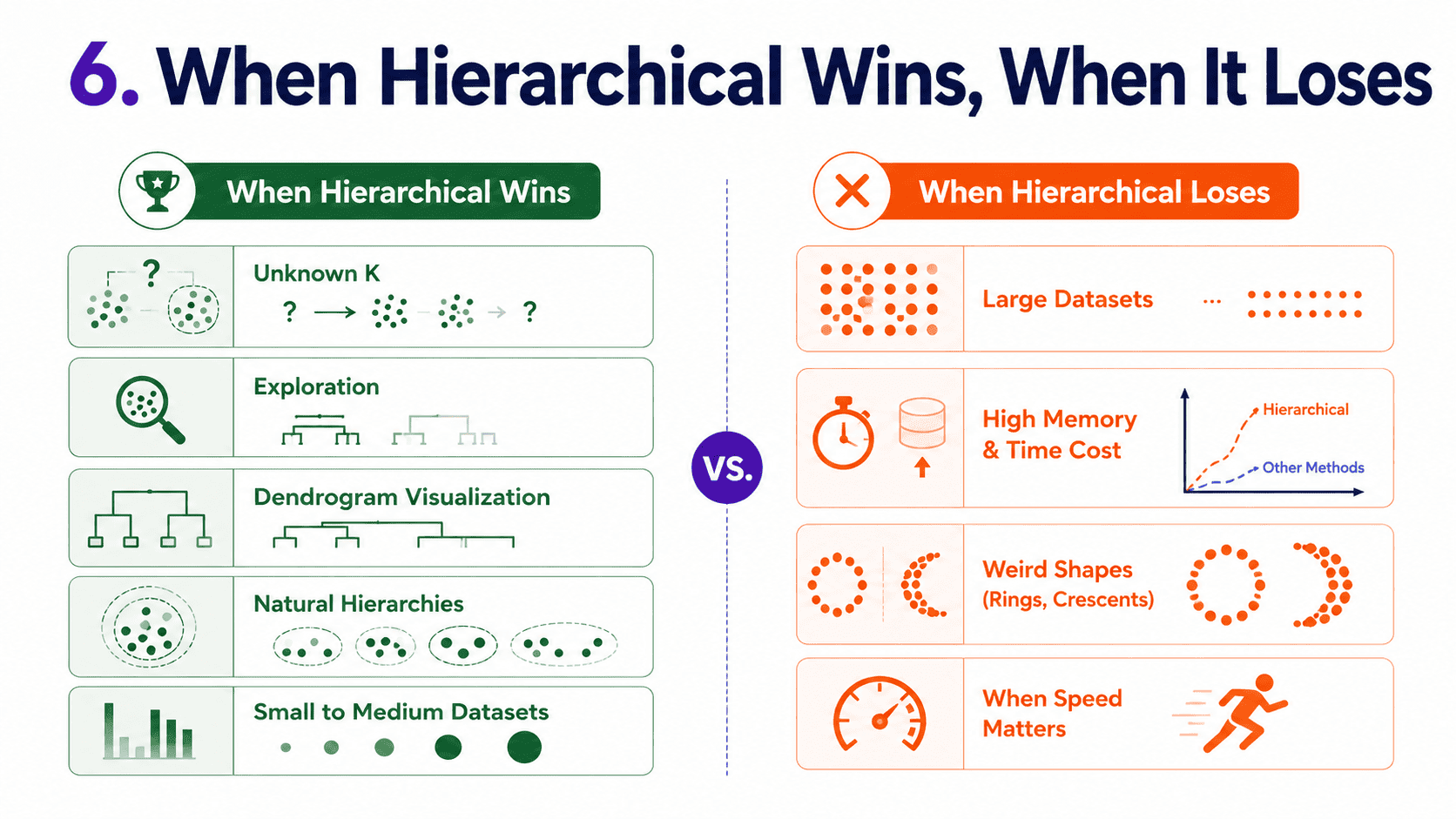
6. When Hierarchical Wins, When It Loses:

It wins when we do not know how many clusters we want and want to explore. When we want a picture of the data's structure. On small-to-medium datasets (up to around 10,000 rows). And when data has natural hierarchical structure (taxonomies, document categories, genetics).

It loses on big datasets, since agglomerative is O(N²) in memory and O(N³) in time. Brutal beyond 10,000 rows. When cluster shapes are weird (rings, half-moons), even Ward struggles. And when we want speed, K-Means is way faster.

7. Hierarchical vs K-Means:

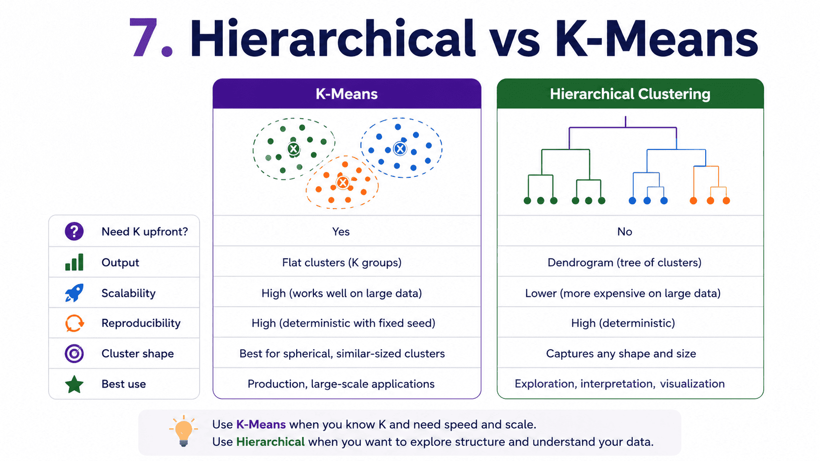A practical pattern. Use hierarchical for exploring data ("how many clusters look reasonable?"), then re-run K-Means with the chosen K for production.

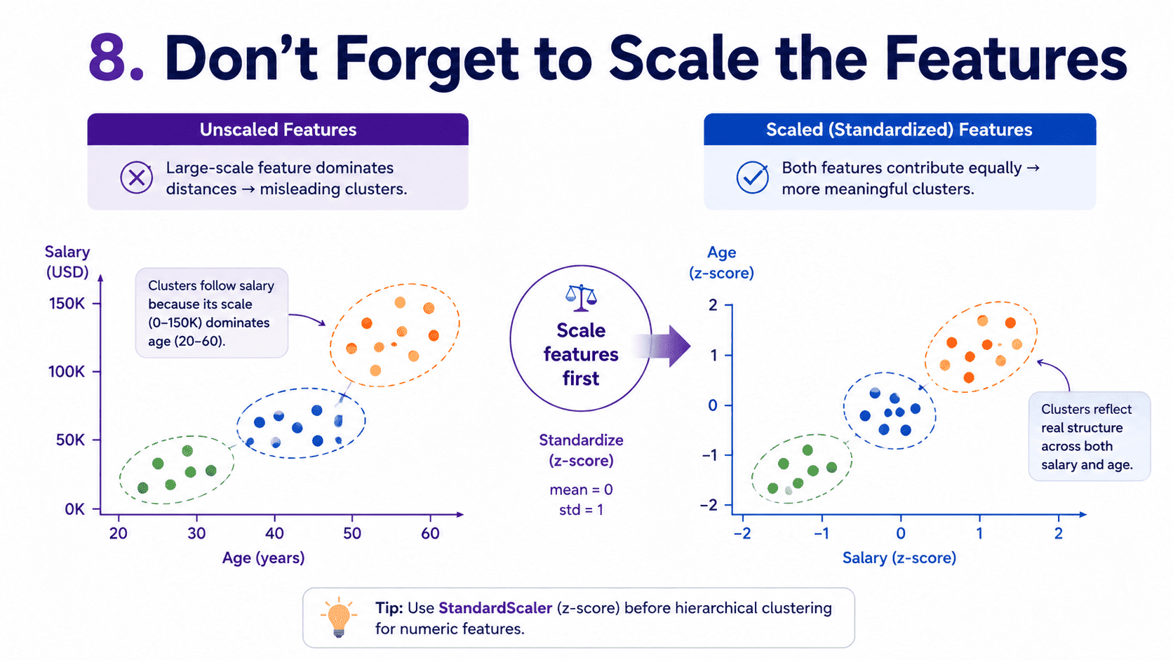
8. Don't Forget to Scale the Features:

Hierarchical clustering uses distances, just like Day 18 Unsupervised Learning & K-Means — Finding Hidden Groups and Day 12 K-Nearest Neighbors — Tell Me Who Your Friends Are. We scale features. Always.

A small thought to sit with.

Suppose our dendrogram has two cuts that both look reasonable, one giving 3 clusters and another giving 5. We are presenting to executives.

How do we decide? A few angles. What is the business need?

Executives often want clusters that map to clear actions. 3 may be easier to explain. Are the 5 clusters meaningfully different? Inspect the feature means in each. If two of the 5 look almost identical, prefer 3.

What does the silhouette score say?

Often it confirms one option over the other. And the dendrogram's superpower is that we can change the cut later, so we show both and recommend one. Stories beat numbers when presenting clustering results.

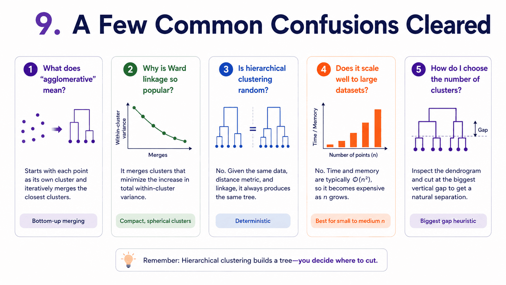
9. A Few Common Confusions Cleared:

• What does "agglomerative" mean? From Latin, "to clump together." Each step clumps two clusters into one.
• Why is Ward linkage popular? It minimises variance increase per merge, so clusters stay tight and balanced, similar to K-Means in spirit but without needing K upfront.
• Is hierarchical clustering deterministic? Yes. Given the same data and linkage, we get the same dendrogram. Unlike K-Means, no random initialisation.
• Why do hierarchical methods scale poorly? Computing all pairwise distances is O(N²) in memory, and the merging is O(N³) in time. Fine for thousands of points, painful for millions.
• Common interview question: "How would you choose the number of clusters in hierarchical clustering?" Inspect the dendrogram. Look for the biggest vertical gap between merges (a big jump means very different clusters were forced to merge). Cut there. Verify with the Day 18 Unsupervised Learning & K-Means — Finding Hidden Groups and business sense.

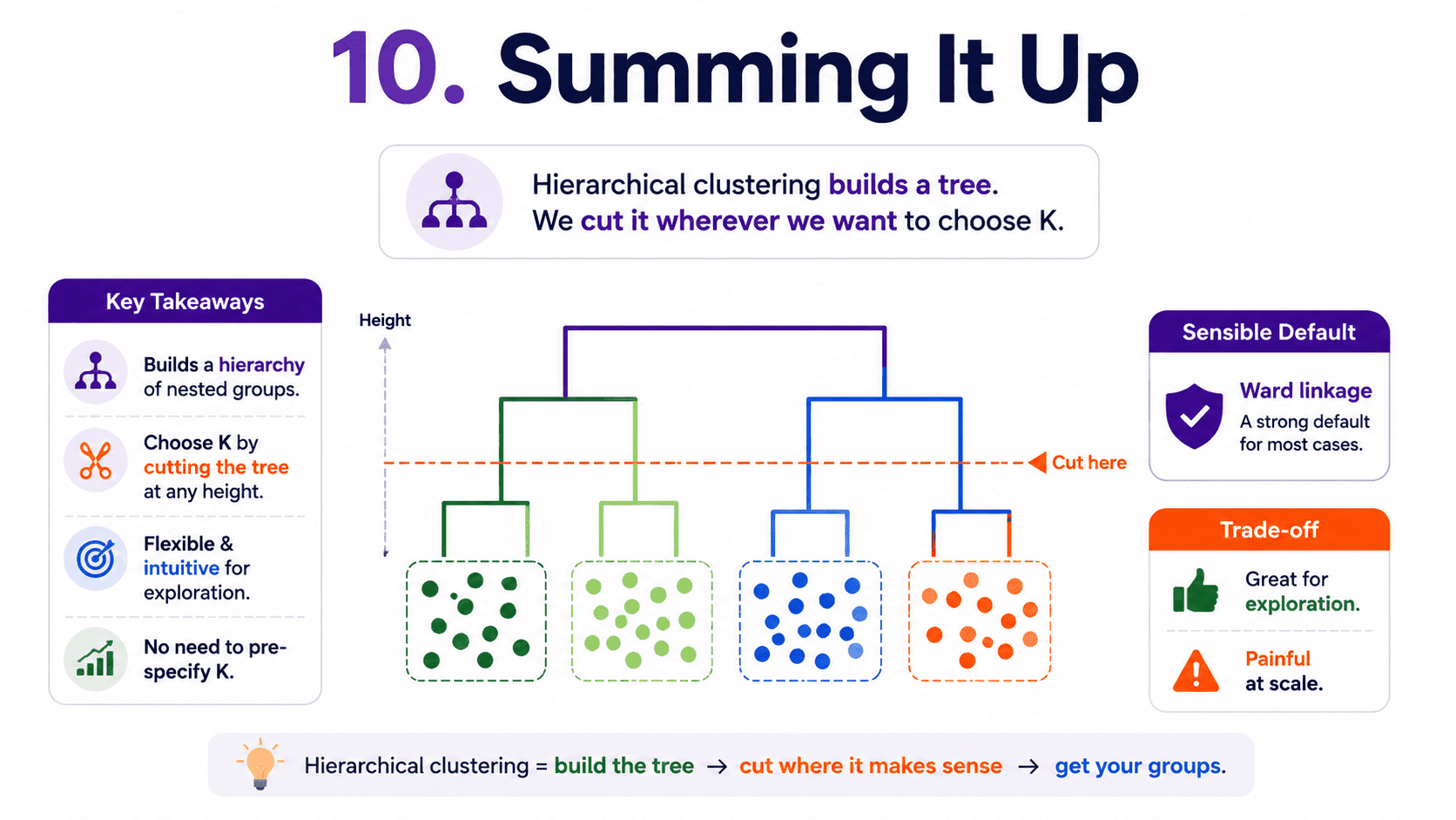
10. Summing It Up:

If we remember one thing from today, it is this: hierarchical clustering builds a tree, and we cut it wherever we want to choose K. Ward linkage is the sensible default. Beautiful for exploration, painful at scale.

Coming Up on Day 20 DBSCAN — Clusters by Density Not Distance

K-Means and Hierarchical both assume our clusters are roughly globular. What if they are crescent-shaped, or our data is full of outliers we want flagged separately? Tomorrow we meet DBSCAN, the clustering algorithm that finds clusters of any shape and automatically discovers noise.

That's all for today. Let's meet up again tomorrow with Day 20.

Thanks for reading.

Cheers!