Day 18: Unsupervised Learning & K-Means — Finding Hidden Groups

Seventeen days of supervised learning, where every example came with an answer attached. Today we cross into a different world.

The model has to find structure in the data on its own, because there are no answers. This is unsupervised learning, and we start with its most famous algorithm: K-Means clustering.

This blog post is a daily learning summary of my ML self-study.

Terms Used Today

Clustering: Finding natural groupings in unlabelled data.

Centroid: The centre of a cluster. K-Means places one centroid per cluster.

WCSS / Inertia: Within-Cluster Sum of Squares. Total squared distance from each point to its cluster centroid. Smaller means tighter clusters.

Elbow method: Plot WCSS vs K and look for the bend.

Silhouette score: For each point, how close it is to its own cluster vs the next-nearest cluster. Ranges from −1 to +1. Higher is better.

K-Means++: Smart initialisation that spreads starting centroids out before the iterations begin.

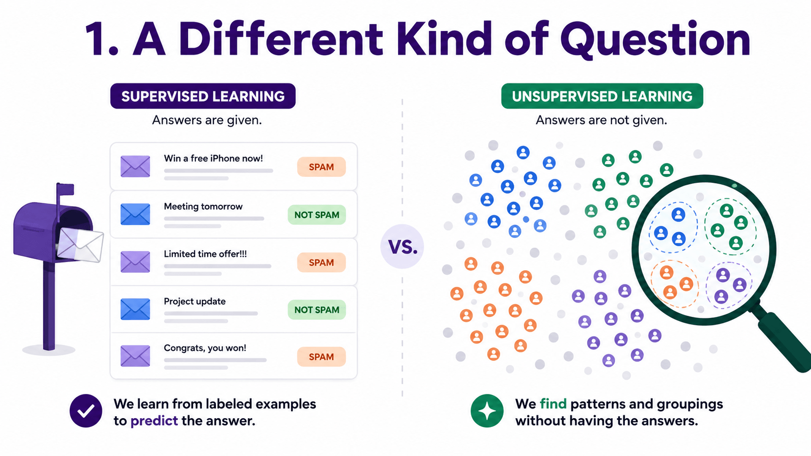
1. A Different Kind of Question:

Supervised learning answered "Given this email, is it spam?". Unsupervised learning answers "Here are ten thousand customers, are there natural groups in here?".

No one tells the algorithm what the groups should be. There is no "correct" answer. The algorithm has to look at the data and find patterns by itself.

This is also closer to how humans explore unfamiliar data. Before we know what question to ask, we want to see what is in the data at all.

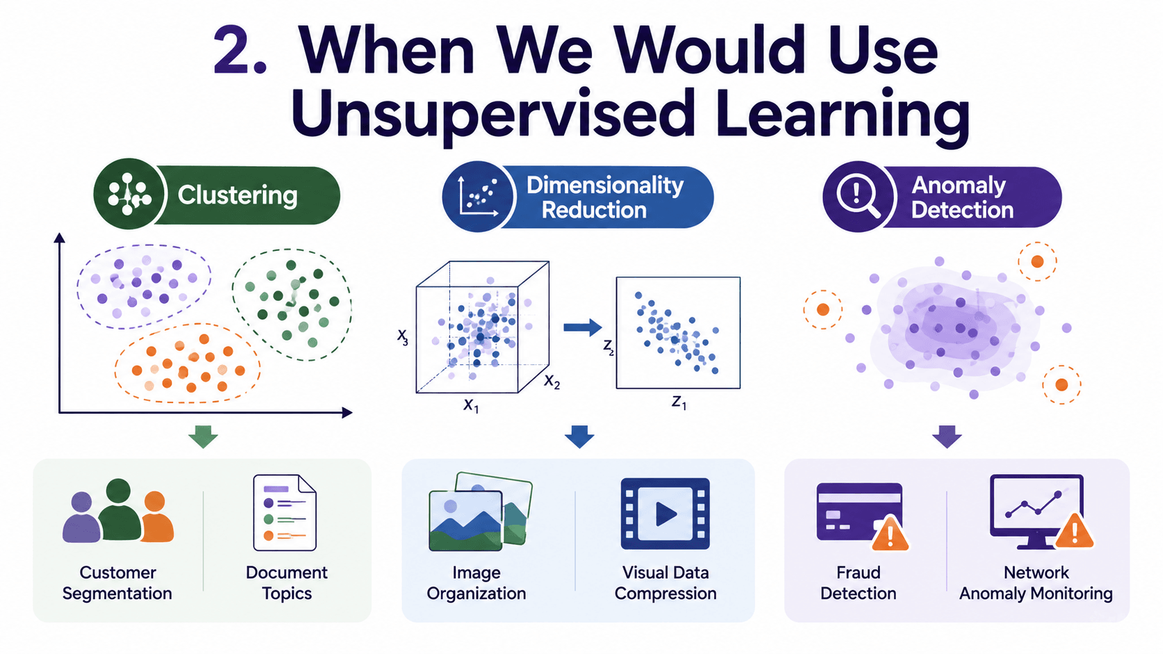
2. When We Would Use Unsupervised Learning:

Three big use cases, which we will meet over the next four days.

Clustering: group similar items (Days 18 to 20).
Dimensionality reduction: squash many features into fewer ([[Day 21 PCA — Shrinking Dimensions Without Losing Meaning|Day 21]]).
Anomaly detection: find what does not fit any pattern.

Some real applications:

Customer segmentation: marketing wants 5 personas, we find 5 clusters of behaviour.
Image organisation: group photos by similarity before labelling.
Topic discovery: what themes appear in 100,000 documents?
Fraud and anomaly detection: flag transactions that do not look like any cluster.

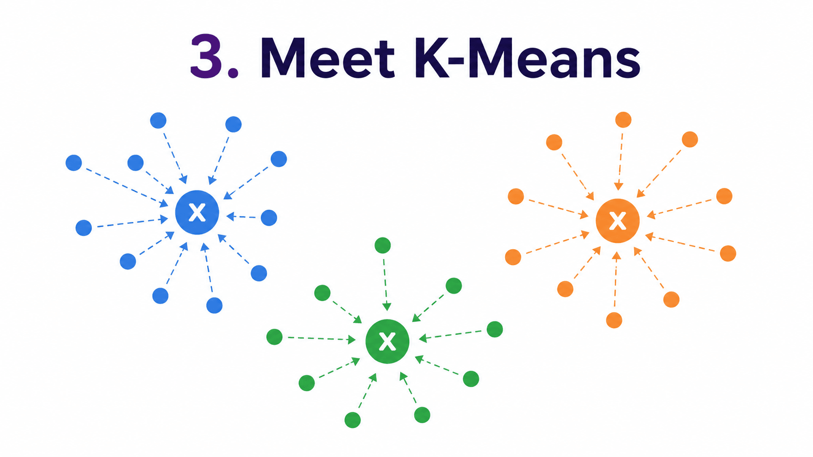
3. Meet K-Means:

The most famous clustering algorithm by far. The "K" is the number of clusters we want, decided in advance.

The premise. Each cluster has a centre (called a centroid). Every data point belongs to the cluster whose centroid is nearest. That is it. The algorithm finds the centroids that "explain" our data best.

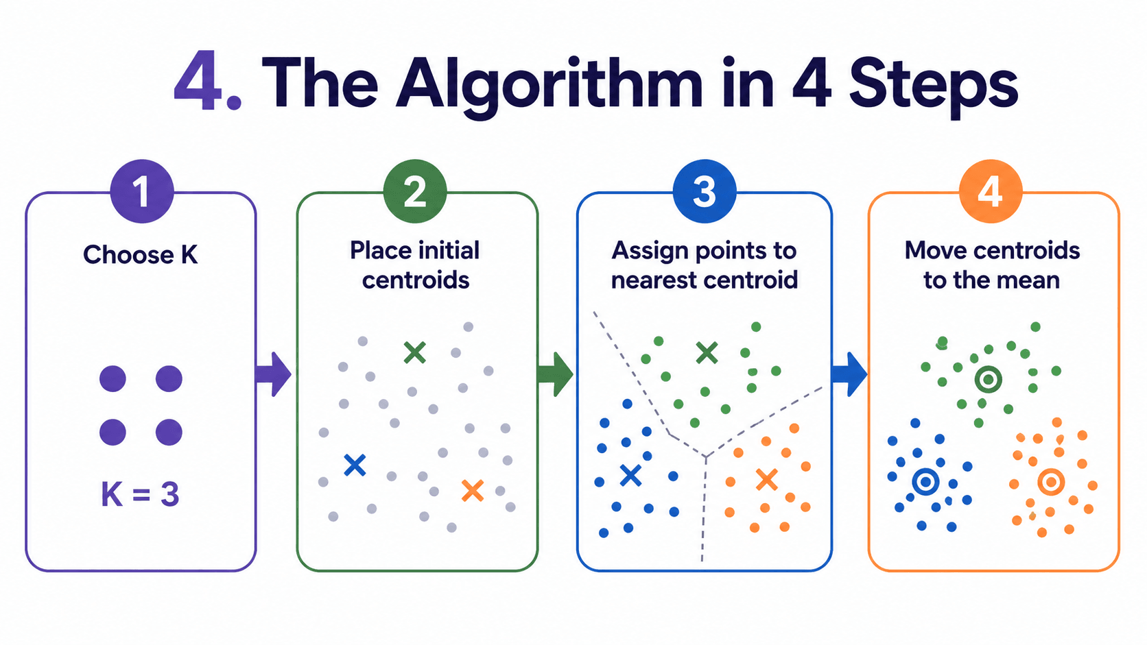
4. The Algorithm in 4 Steps:

Pick K. Decide how many clusters we want, say K = 3.
Place centroids. Drop K random points into our data as initial centroids.
Assign. Every data point joins its nearest centroid, forming K groups.
Update. Move each centroid to the average position of its assigned points.

Repeat steps 3 and 4 until the centroids stop moving. Picture it like magnets. Each centroid pulls in nearby points, then re-centres itself among them. The centroids drift around until they settle.

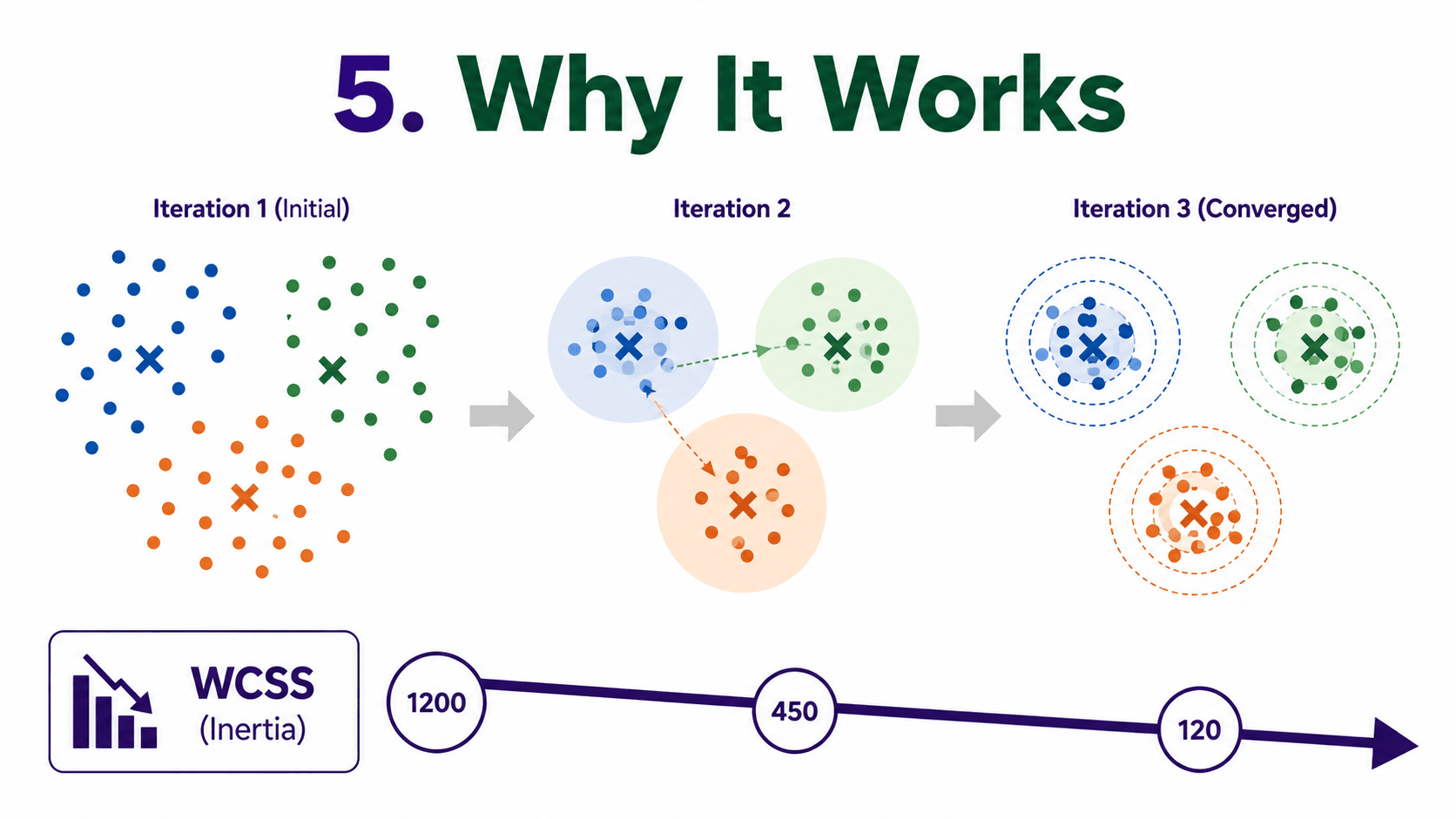
5. Why It Works:

At each iteration, the algorithm reduces the Within-Cluster Sum of Squares (WCSS): the total squared distance from points to their cluster centres.

K-Means minimises the spread inside each cluster.

Each iteration is guaranteed not to make things worse. Eventually, the algorithm converges. The catch. It converges to a local minimum that depends on the initial centroid placement. Different random starts can give different final clusters. We will deal with this in a moment.

6. How to Pick K (The Elbow Method):

The big practical question. K is not learned; we have to choose it.

We try several K values (1, 2, 3, ..., 10). For each, we compute the WCSS. Plot it. 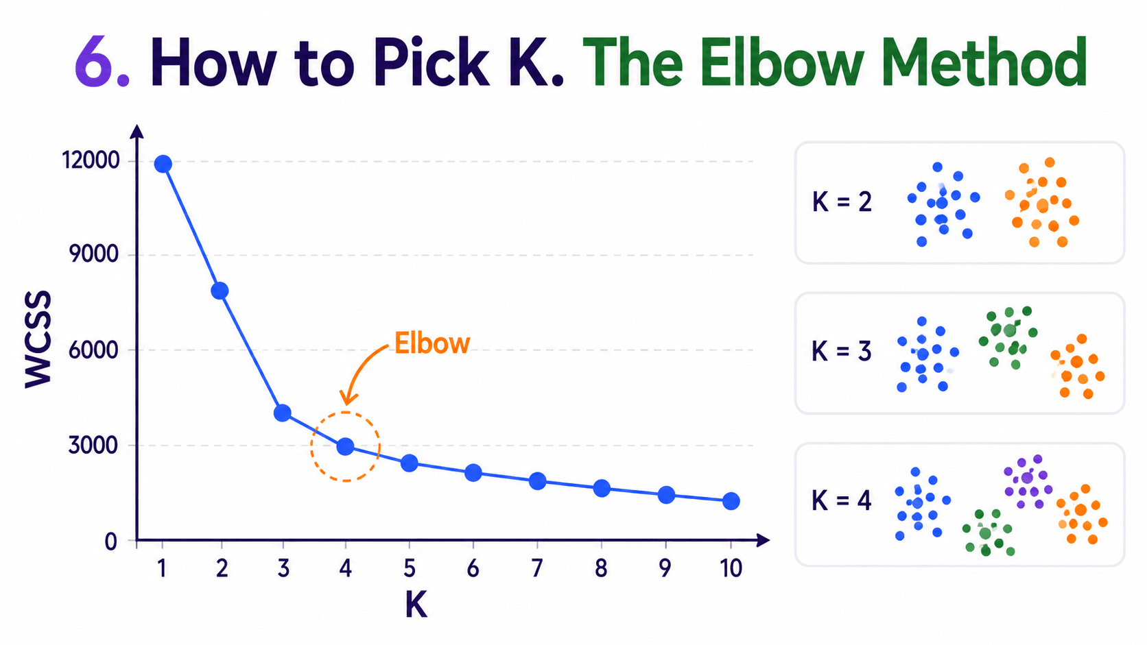The curve always drops, because more clusters always fit better. But it usually has a clear elbow: the K beyond which extra clusters add very little. Pick K at the elbow. Around 3 in this picture.

from sklearn.cluster import KMeans
wcss = []
for k in range(1, 11):
    km = KMeans(n_clusters=k, n_init=10, random_state=42)
    km.fit(X)
    wcss.append(km.inertia_)

Plot wcss against K. Look for the bend.

The elbow is not always sharp. When in doubt, we use the silhouette score as a second opinion.

7. Silhouette Score:

For each point, compute two things:

a = average distance to other points in its own cluster.
b = average distance to points in the next-nearest cluster.

Then:

silhouette = (b − a) / max(a, b)

The result is between −1 and +1.

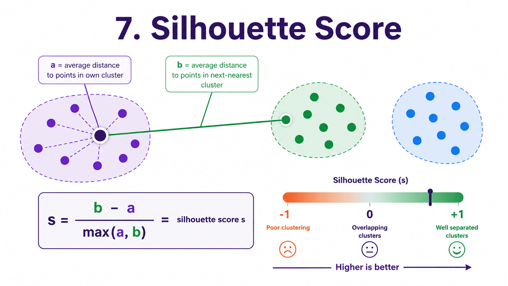
+1 → point is much closer to its own cluster than the neighbour. Perfect fit.
0 → point is on the boundary between two clusters.
−1 → point is closer to the neighbour cluster than its own. Wrongly assigned.

Average the silhouette over all points and we get a single number. We try several K values and pick the K with the highest average silhouette. It often agrees with the elbow. When they disagree, silhouette tends to be more reliable.

from sklearn.metrics import silhouette_score
sil = silhouette_score(X_scaled, labels)
print(sil)

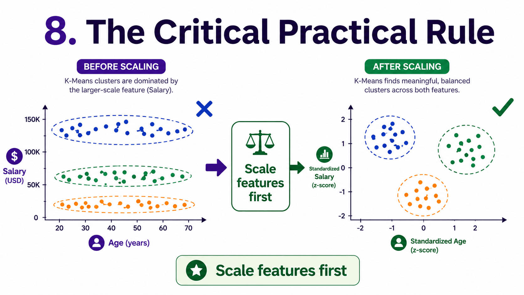
8. The Critical Practical Rule:

Always scale features before K-Means.

Just like in Day 12: K-Nearest Neighbors — Tell Me Who Your Friends Are, K-Means uses Euclidean distances. Features on bigger scales dominate. A salary feature in dollars will completely drown out an age feature in years. Always wrap K-Means in a pipeline with StandardScaler.

9. Initial Centroid Placement:

Bad initialisation can give bad clusters. To fix this, we run K-Means multiple times with different random starts and keep the result with lowest WCSS. sklearn does this with n_init=10 (the default), running 10 random starts behind the scenes.

There is also a smarter method called K-Means++ that spreads initial centroids out.

sklearn uses K-Means++ by default. We do not need to set anything.

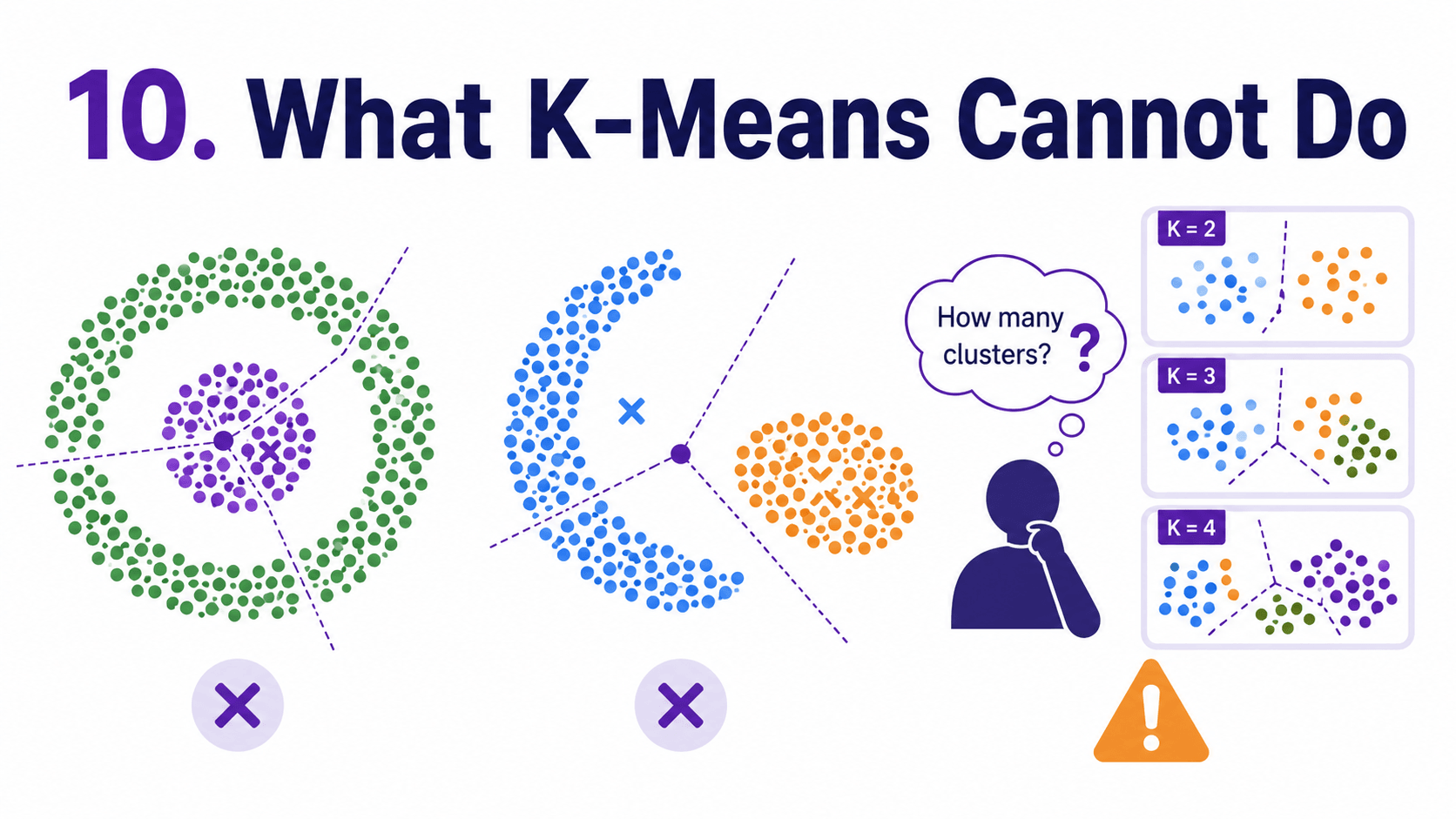
10. What K-Means Cannot Do:

K-Means makes three big assumptions.

Clusters are roughly spherical. Bad for crescent or ring-shaped clusters.
Clusters are roughly equal-sized. It will split big clusters and merge small ones.
We know K in advance. There is no automatic way to discover the right number.

If our data violates these assumptions, we look at Day 19 Hierarchical Clustering — A Family Tree for Data (Hierarchical) and Day 20 DBSCAN — Clusters by Density Not Distance (DBSCAN). Both lift different limitations.

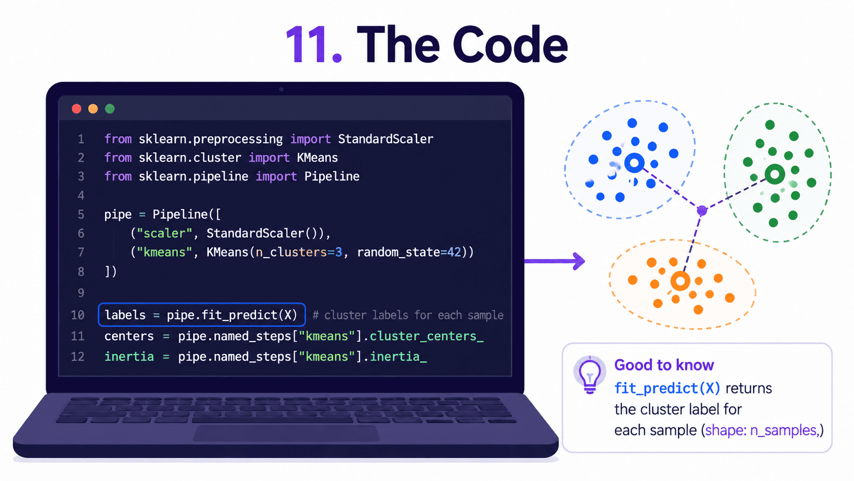
11. The Code:

from sklearn.preprocessing import StandardScaler
from sklearn.cluster import KMeans
from sklearn.pipeline import Pipeline

pipe = Pipeline([
    ('scaler', StandardScaler()),
    ('kmeans', KMeans(n_clusters=4, n_init=10, random_state=42))
])

clusters = pipe.fit_predict(X)
print(pipe.named_steps['kmeans'].cluster_centers_)   # the centroids
print(pipe.named_steps['kmeans'].inertia_)            # the WCSS

fit_predict returns the cluster label (0 to K minus 1) for each row.

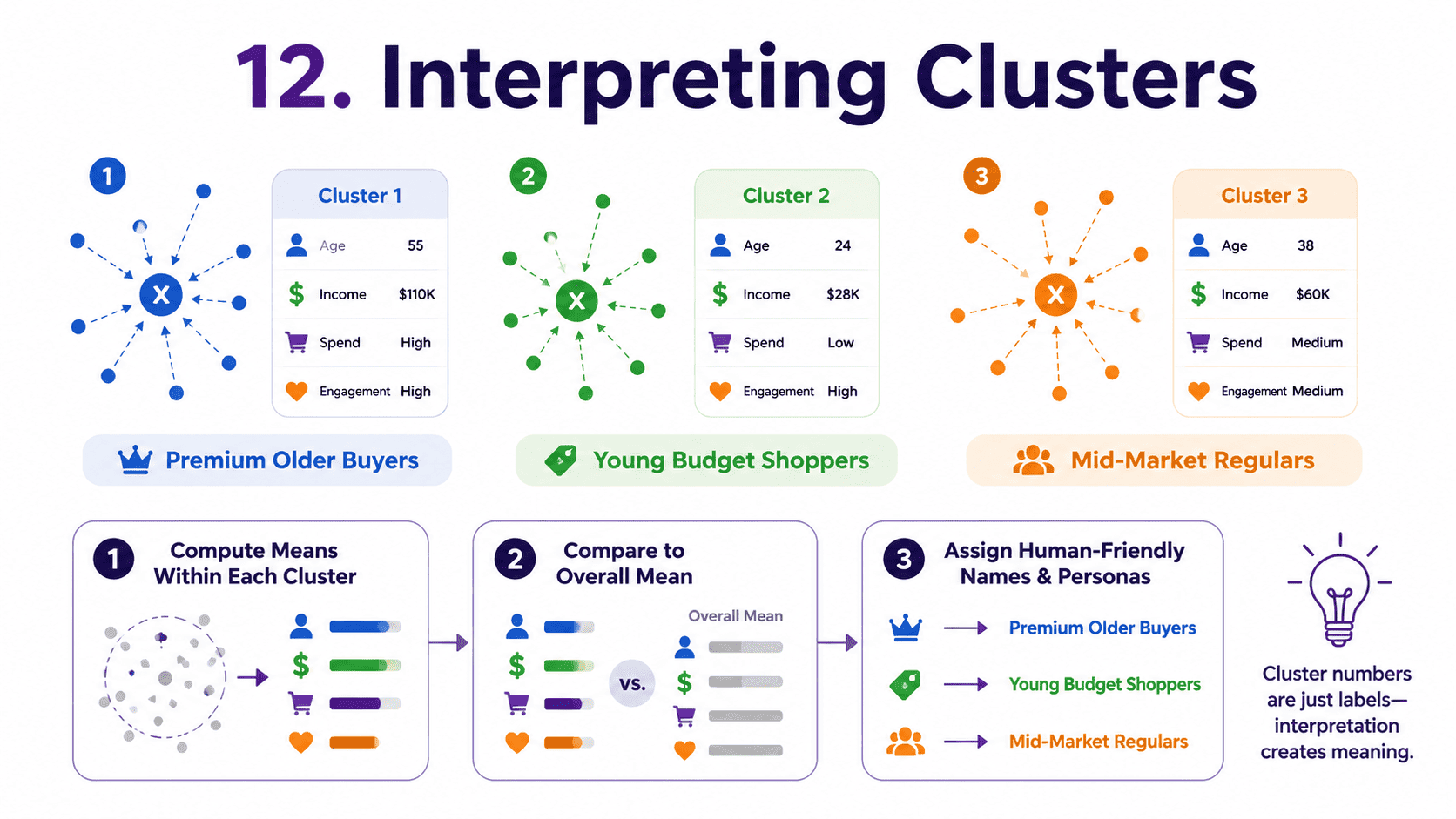
12. Interpreting Clusters:

After K-Means runs, the labels are just numbers. To make sense of them:

Compute the mean of each feature within each cluster.
Compare to the overall mean.
Name the clusters based on the dominant differences.

For example, "Cluster 2 has higher income and older customers, let us call it Premium Older Buyers." Naming clusters is half art, half data. Senior data scientists are good at it.

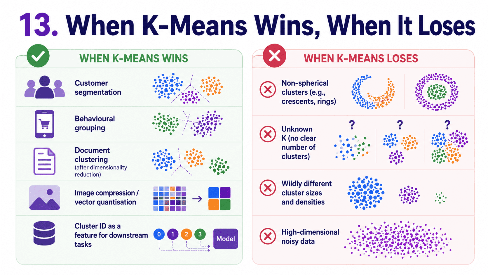
13. When K-Means Wins, When It Loses:

It wins for customer segmentation and behavioural grouping, for document clustering after dimensionality reduction, for vector quantisation (image compression), and for preprocessing for downstream tasks (using cluster ID as a new feature).

It loses when cluster shapes are not spherical (use DBSCAN). When we do not know K (use Hierarchical or DBSCAN). When clusters have wildly different sizes. And when data is high-dimensional and noisy (reduce dimensions first via Day 21 PCA — Shrinking Dimensions Without Losing Meaning.

A small thought to sit with.

Suppose our boss says "give me three customer segments."

We run K-Means with K = 3 and get the clusters. But the elbow method suggests K = 6 looks better.

What do we do? We talk to our boss.

Three clusters is a business requirement, not a statistical one. We can either use K = 3 if business strongly needs three (presentations, campaigns), or show K = 6 first and group them into 3 super-clusters with human reasoning, or use K = 6 and pitch the extra granularity.

ML often hits these business-vs-data tensions, and we should not blindly pick the elbow. Always understand the why.

14. A Few Common Confusions Cleared:

Is K-Means deterministic? No. Initial centroids are random. We use random_state and n_init for reproducible runs.
What is "inertia"? sklearn's name for within-cluster sum of squared distances (WCSS). Lower is better, but adding clusters always lowers it, which is why we use the elbow method.
Why must we scale features? K-Means uses Euclidean distance. Without scaling, large-magnitude features dominate.
Can K-Means handle categorical features? Not natively. Euclidean distance on one-hot encodings is dodgy. Use K-Modes (variant for categorical) or convert categoricals carefully.
Common interview question: "How do you choose K in K-Means?" Elbow method first (plot WCSS vs K, find the bend). Verify with silhouette score (average over all points, pick the K with the highest). Sometimes business constraints override both.

15. If This Came In An Interview:

A few questions to be ready for, with one-line answers.

How does K-Means work? Pick K centroids randomly, assign each point to its nearest centroid, move each centroid to the mean of its assigned points, repeat until the centroids stop moving.
How do you choose K? Elbow method first (plot WCSS vs K, look for the bend). Verify with the silhouette score (pick K with the highest average). Sometimes business constraints override both.
What is the silhouette score? For each point, how close it is to its own cluster vs the next-nearest cluster. Ranges from −1 to +1. Average over all points gives a single quality number.
Why must features be scaled before K-Means? Because it uses Euclidean distance. Without scaling, large-magnitude features dominate.
What are K-Means' main assumptions? Clusters are roughly spherical and equal-sized, and K is known in advance. When these break, use DBSCAN or Hierarchical instead.
Is K-Means deterministic? No, initial centroid placement is random. Use random_state and n_init for reproducibility. sklearn's K-Means++ default reduces sensitivity to initialisation.

16. Summing It Up:

If we remember one thing from today, it is this: K-Means is just "assign to nearest centroid, recompute centroid, repeat." Choose K with the elbow method or silhouette score. Always scale features. Works beautifully for spherical, equal-sized clusters, and struggles with weird shapes, which Days 19 and 20 will fix.

Coming Up on Day 19 Hierarchical Clustering — A Family Tree for Data

K-Means insisted we know K in advance. Tomorrow we meet a clustering algorithm that builds a whole family tree of clusters and lets us choose K at the end, by simply cutting the tree at the right height. Welcome to Hierarchical Clustering.

That's all for today. Let's meet up again tomorrow with Day 19.

Thanks for reading.

Cheers!