Day 17: Support Vector Machines — Drawing the Widest Lane

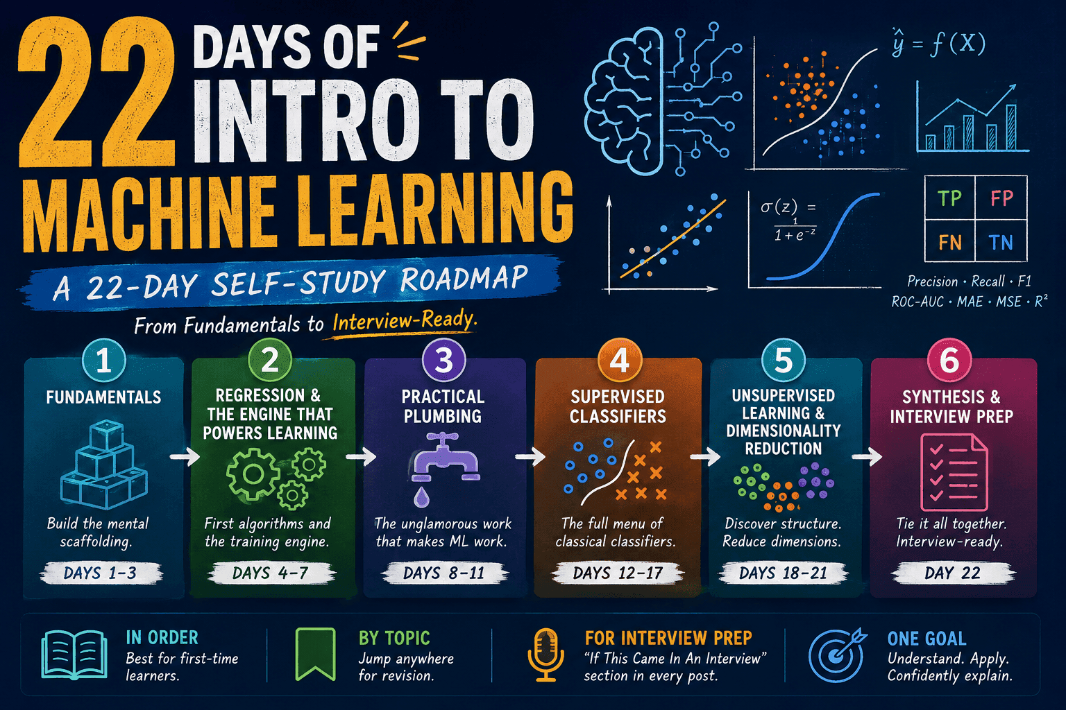
Our last supervised algorithm. Before deep learning conquered everything in the 2010s, SVMs were the king of classification. They are still genuinely useful for small-to-medium problems, and they give us the cleanest illustration of one of the most beautiful ideas in ML: the kernel trick.

This blog post is a daily learning summary of my ML self-study.

Terms Used Today

Margin: The gap between the boundary and the nearest points of each class.

Support vectors: The boundary-defining points. Everything else is irrelevant for prediction.

Soft margin (C): Controls how harshly we punish misclassification. Smaller C means a wider, more tolerant margin.

Kernel: A function that lets SVM act as if data were in a higher dimension, without actually projecting it.

RBF kernel: The popular default kernel. Produces flexible, curved boundaries.

gamma: Controls how "wiggly" the RBF boundary can be (high = bumpy, low = smooth).

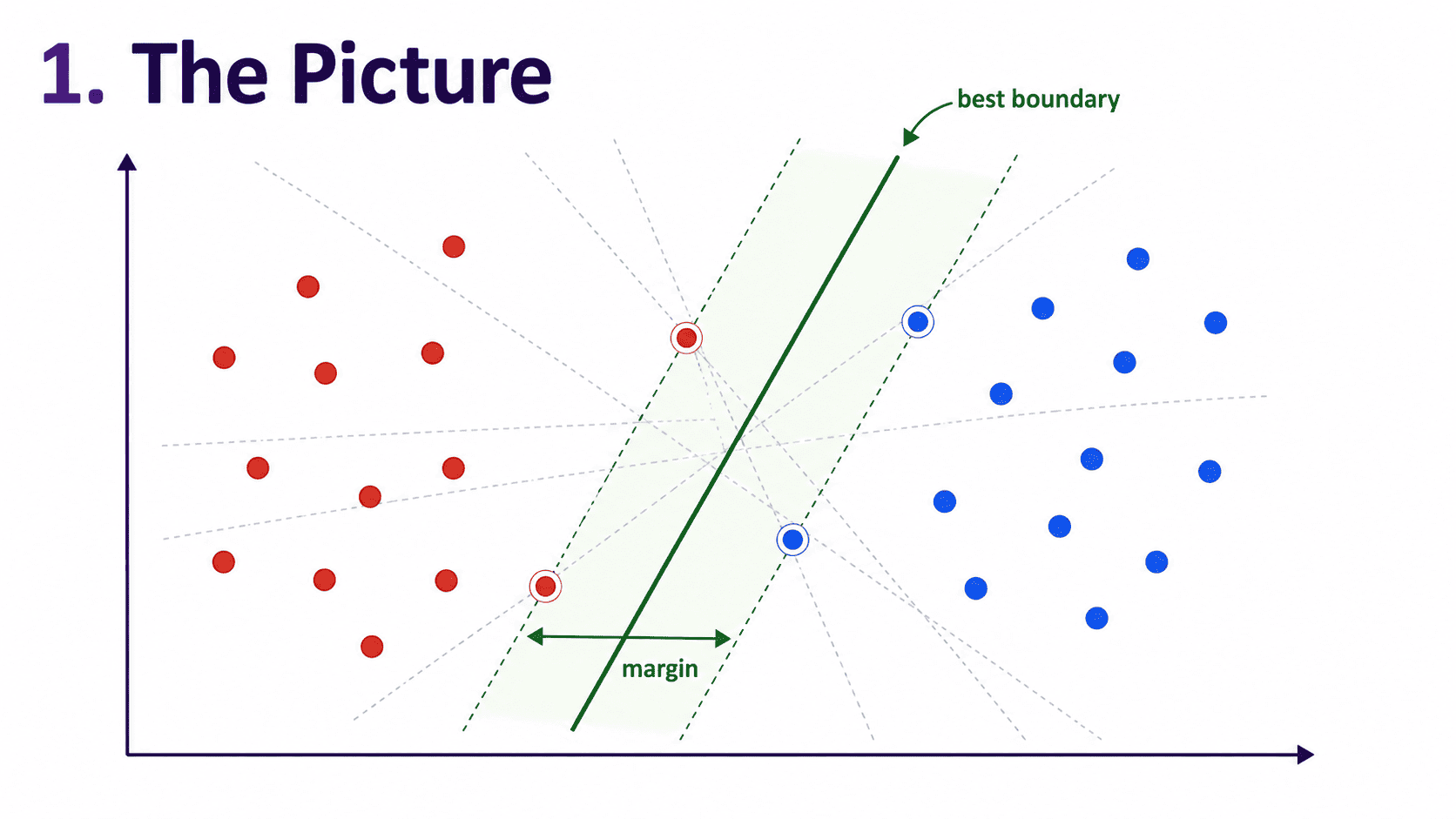
1. The Picture:

Imagine two groups of points on a piece of paper.

Red dots on the left.
Blue dots on the right.

We want to draw a line that separates them. How many such lines exist? Infinitely many. Which one is best?

SVM's answer is the line that is as far from both groups as possible.

Pick the boundary that leaves the widest possible gap between the classes.

That widest gap is called the margin. SVM is, fundamentally, the Maximum Margin Classifier.

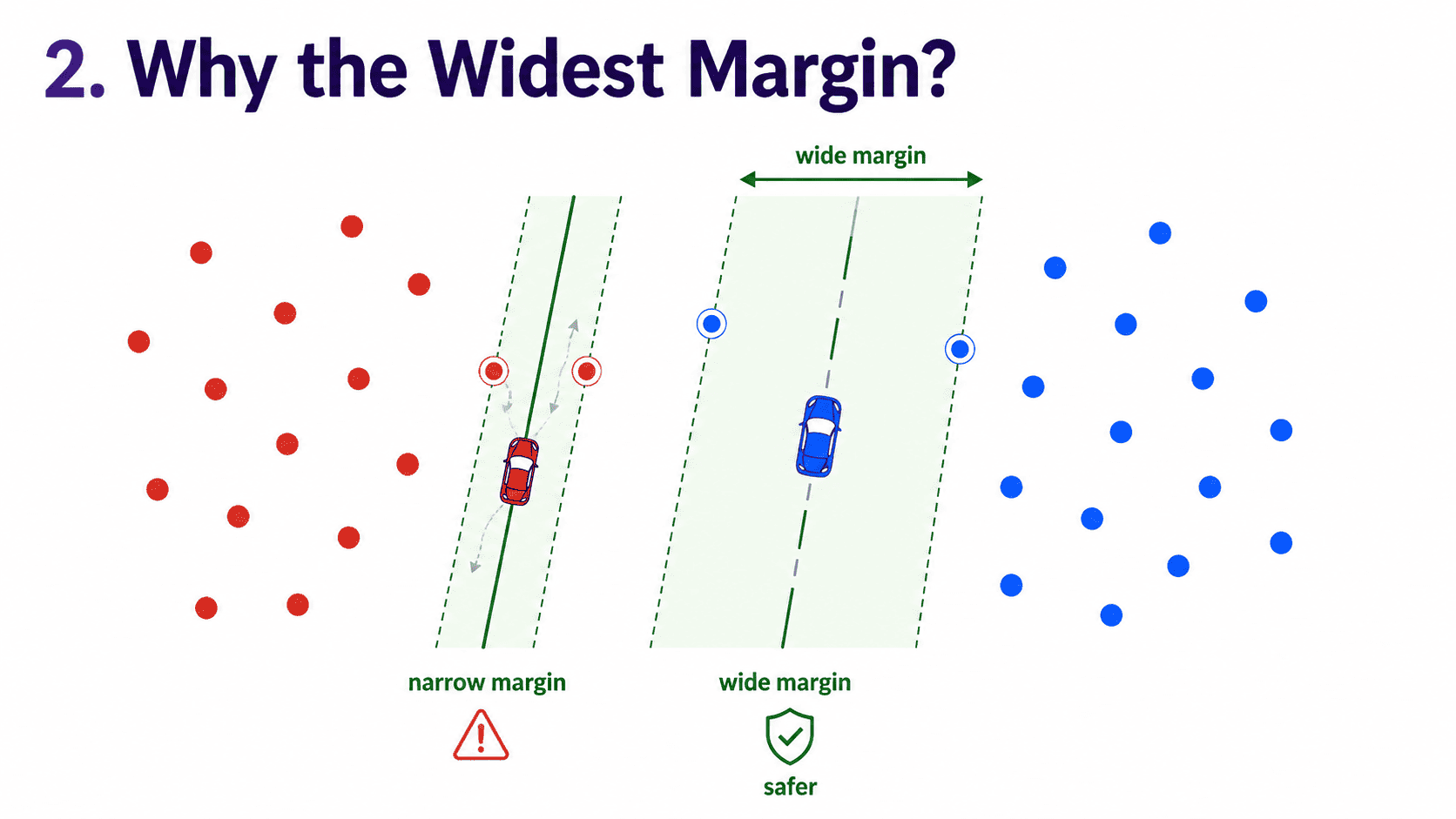
2. Why the Widest Margin?

A boundary with a tiny margin is dangerous. A new point near the line could be misclassified by a hair. A boundary with a wide margin is safe; there is room to be wrong.

Think of it like driving. A narrow lane means a small wobble sends us off-road. A wide lane gives us cushion. SVM picks the widest lane between the classes.

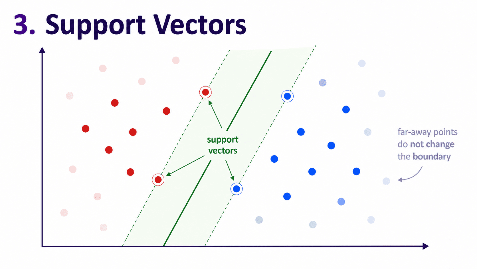
3. Support Vectors:

Look at the boundary SVM picks. Which points actually matter?

Only the points closest to the boundary, the ones touching the edge of the margin. These are the support vectors.

Everything else is irrelevant. Move a far-away point a little and the boundary does not change. Move a support vector and the boundary jumps.

This makes SVM memory-efficient (only the support vectors matter for prediction) and robust to far-away points (they do not affect the decision).

The name "Support Vector Machine" comes from these special boundary points.

4. What If the Data Is Not Cleanly Separable?

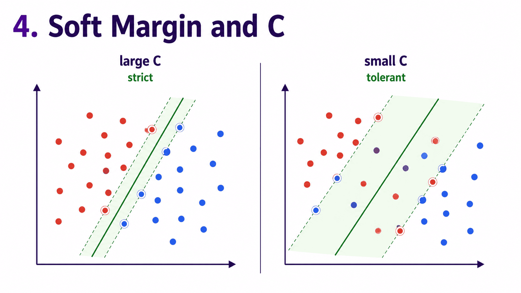
Real-world data is not always cleanly separable. Some red dots might sit on the blue side, and vice versa. SVM allows some violations. It introduces a soft margin.

The line can misclassify a few points if doing so makes the margin wider overall. The balance is controlled by a hyperparameter called C.

Large C → punish misclassification heavily → narrow margin, fewer training mistakes. (Risk: overfit.)
Small C → tolerate misclassification → wider margin, more smoothing. (Risk: underfit.)

C is the regularisation knob for SVM.

5. The Kernel Trick (Intuition Only):

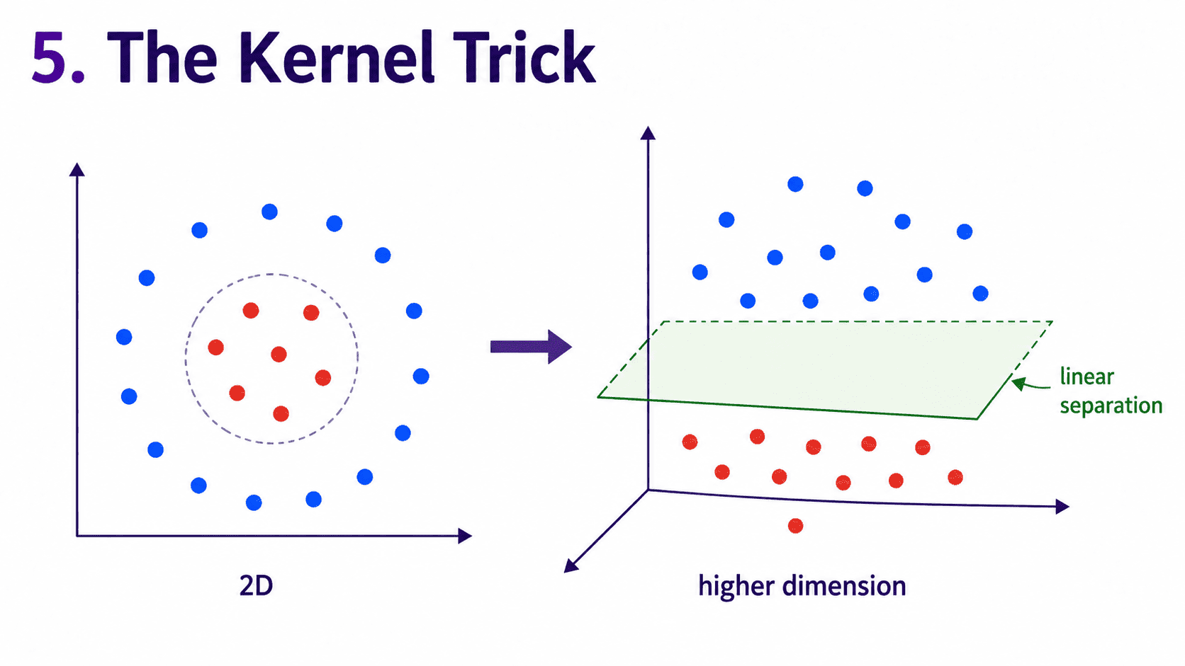
Here is the magic. What if the data cannot be separated by any straight line?

Picture two circles. An inner ring of red dots and an outer ring of blue. No line in 2D can separate them.

The kernel trick says: lift the data into a higher dimension where a flat boundary becomes possible.

For circles, transform (x, y) into (x, y, x² + y²). The third dimension is "distance from origin." Now the inner ring is low, the outer ring is high, and a flat plane in 3D separates them cleanly.

In general, any messy 2D problem can be untangled if we go up enough dimensions. The genius of the kernel trick is that SVM does this implicitly, without ever literally computing the higher dimensions.

It uses a kernel function to compute similarities in the higher space directly. Mathematically clever, computationally efficient.

Common kernels:

Linear: no transformation, just a straight-line boundary.
Polynomial: quadratic, cubic boundaries.
RBF (Radial Basis Function): the popular default; can carve almost any shape.
Sigmoid: similar to neural networks (less commonly used).

The RBF kernel is the Swiss Army knife. Start there.

6. Two Knobs to Tune:

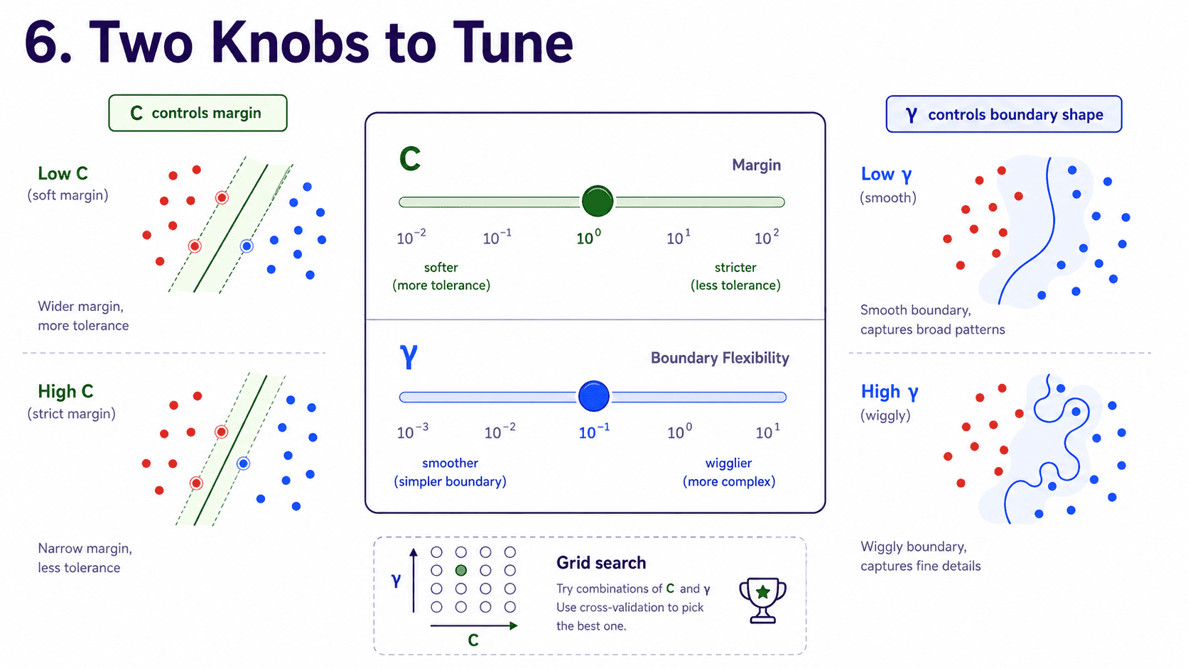
For SVM with the RBF kernel, the two main knobs are:

C: the softness of the margin (regularisation).
gamma: how "wiggly" the boundary can be (low gives smooth, high gives bumpy).

We tune both together using GridSearchCV (Day 10 Cross-Validation & Hyperparameter Tuning).

A common starting grid:

{'C': [0.1, 1, 10, 100], 'gamma': [0.001, 0.01, 0.1, 1]}

7. The Code:

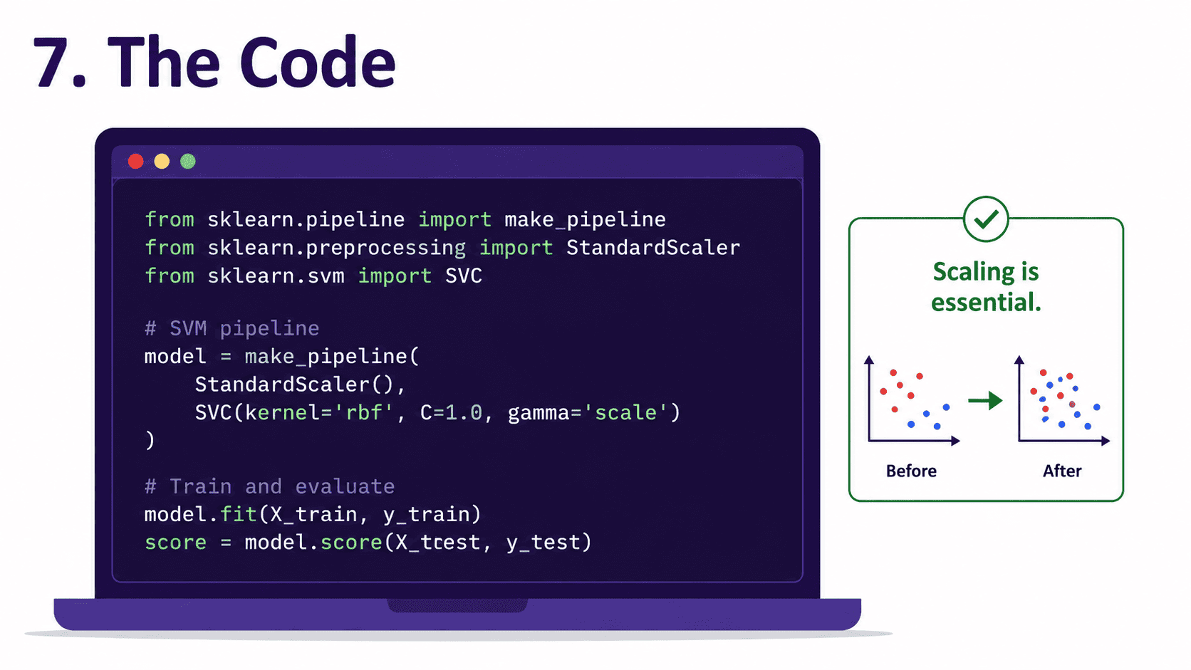
from sklearn.svm import SVC
from sklearn.preprocessing import StandardScaler
from sklearn.pipeline import Pipeline

pipe = Pipeline([
    ('scaler', StandardScaler()),    # essential
    ('svm', SVC(kernel='rbf', C=1.0, gamma='scale'))
])

pipe.fit(X_train, y_train)
print(pipe.score(X_test, y_test))

gamma='scale' is sklearn's smart default. Always scale features before SVM.

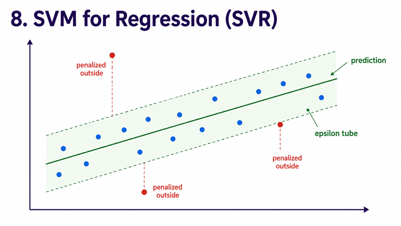
8. SVM for Regression (SVR):

There is a regression flavour, called SVR (Support Vector Regression). The idea flips. Instead of finding the widest margin between classes, SVR finds a fit where most points sit within an epsilon (ε) tube around the prediction line.

Anything inside the tube counts as zero error; only points outside the tube are penalised. The hyperparameter ε sets how wide the tube is. Less commonly used than SVM for classification, but worth knowing it exists.

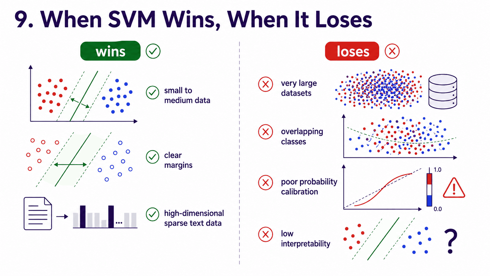
9. When SVM Wins, When It Loses:

It wins on small-to-medium datasets (up to ~50k rows), on clean class boundaries with clear margins, on high-dimensional but sparse data (text classification used to use SVM heavily), and when we need a strong classifier but lack the data for boosting to shine.

It loses on very large datasets (training scales poorly, between O(n²) and O(n³)). On heavily overlapping classes (boosted trees usually do better).

When we need probabilities (SVM does not naturally give well-calibrated ones; Platt scaling helps but is hacky). And when we need interpretability, since SVM boundaries are not human-readable (especially with kernels).

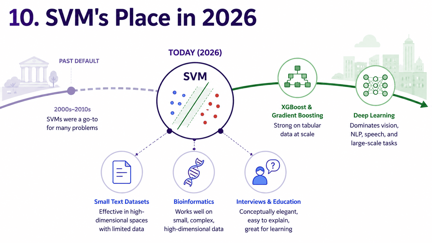
10. SVM's Place in 2026:

A decade ago, SVM was the default classifier. Then XGBoost arrived for tabular and deep learning arrived for everything else. SVM still shows up in:

Text classification on smaller datasets.
Bioinformatics (small sample sizes, very high dimensions).
Interview questions! We should expect at least one SVM question.

For interviews, we should be able to explain max margin, support vectors, soft margin (C), and the kernel trick without panicking.

A small thought to sit with. Suppose we are classifying handwritten digits using SVM. With a linear kernel, we get 87% accuracy. With an RBF kernel, we get 96% but training takes 10× longer.

What does the gap tell us, and what is the tradeoff?

The gap tells us that the boundary between digit classes is non-linear. RBF buys us that flexibility, at the cost of compute. On a small dataset, we take RBF and the extra accuracy. On a big dataset where SVM is already slow, the gap might be worth it, or we might be better off switching to XGBoost or a neural net.

11. A Few Common Confusions Cleared:

Why scale features for SVM? Because margins are measured in distance. Features on bigger scales would dominate the geometry, just like in [[Day 12 K-Nearest Neighbors — Tell Me Who Your Friends Are|KNN]].
SVM vs Logistic Regression? Both produce linear boundaries. Logistic regression minimises log loss (probabilistic). SVM maximises the margin (geometric). For linearly separable data, both work similarly. SVM tends to be more robust to outliers far from the boundary.
Is SVM still relevant? For tabular, mostly no, since XGBoost dominates. For text with TF-IDF features and small data, yes. For interviews, definitely.
Why does SVM not give probabilities by default? Its decision is "which side of the line," not a probability. sklearn can fit a logistic curve to the decision values (Platt scaling, probability=True) to fake probabilities. Do not rely on these as truly calibrated.
Common interview question: "What is the kernel trick?" A way to compute as if we had projected the data into a higher-dimensional space, where a non-linear boundary becomes linear, without actually projecting it. We only compute similarity between pairs of points using a kernel function.

12. If This Came In An Interview:

A few questions to be ready for, with one-line answers.

What does SVM optimise for? The widest possible margin between classes. Among all valid separating boundaries, it picks the one furthest from the closest training points.
What are support vectors? The training points closest to the boundary. They are the only ones that define it; everything else is irrelevant for prediction.
What is the kernel trick? A way to compute as if we projected data into a higher-dimensional space (where a non-linear problem becomes linear), without actually projecting it.
What does C control? The softness of the margin. Large C punishes misclassification harshly (narrow margin). Small C tolerates misclassification (wider margin).
SVM vs Logistic Regression? Both produce linear boundaries. Logistic Regression minimises log loss (probabilistic). SVM maximises the margin (geometric). SVM is more robust to far-away outliers.
Does SVM give probabilities? Not natively. sklearn can fit a logistic curve to decision values (Platt scaling) to estimate them, but they are not well-calibrated.
Why scale features for SVM? Because margins are measured in distance. Bigger-scale features would dominate the geometry.

13. Summing It Up:

If we remember one thing from today, it is this: SVM draws the widest possible lane between the two classes. Only the closest points (support vectors) define that lane. The soft margin (controlled by C) allows some misclassification, and the kernel trick lets SVM draw non-linear boundaries by implicitly working in higher dimensions. Powerful for small-to-medium problems, with RBF as the safe default kernel.

Coming Up on Day 18 Unsupervised Learning & K-Means — Finding Hidden Groups

That wraps up supervised learning. Tomorrow we step into a completely different world: data with no answer key, where the model has to find structure on its own. We will meet the most widely used clustering algorithm, K-Means, and the elbow method that helps decide how many groups exist.

That's all for today. Let's meet up again tomorrow with Day 18.

Thanks for reading.

Cheers!