Day 16: Gradient Boosting & XGBoost — Learning from Mistakes

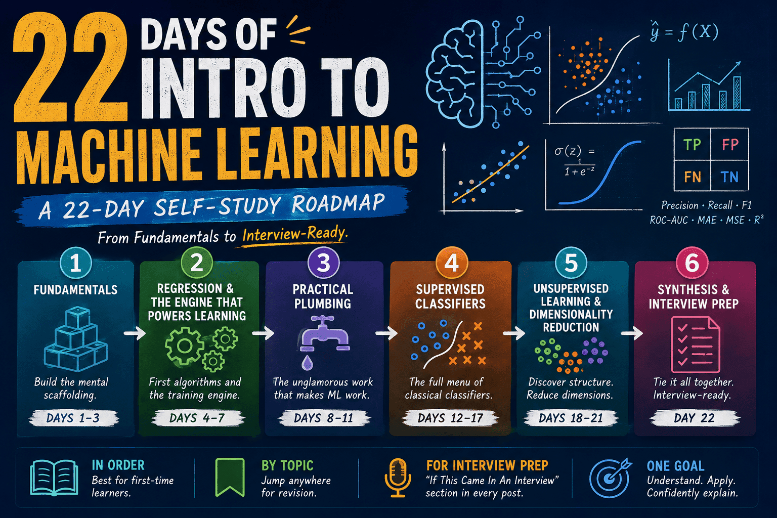
Random Forest trained 500 trees independently and averaged them. Today we meet a smarter idea. Train trees one at a time, with each new tree focused on fixing the mistakes of the previous ones. This is gradient boosting, the algorithm that has dominated Kaggle competitions for over a decade and is one of the strongest defaults in tabular ML.

This blog post is a daily learning summary of my ML self-study.

Terms Used Today

Boosting: Train models sequentially, each new one correcting the previous ones' mistakes.

Residual: The error between predicted and actual values. Each new tree tries to fit the leftover residuals.

Learning rate: Shrinks each tree's contribution. Small rate plus many trees usually gives the best results.

Early stopping: Halt training when validation score stops improving.

XGBoost / LightGBM / CatBoost: The three most-used gradient boosting libraries.

scale_pos_weight: XGBoost's class-imbalance knob.

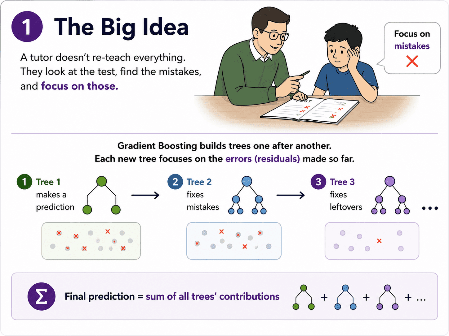
1. The Big Idea:

A tutor helping a student does not re-teach the whole subject. They look at the test, find the questions the student got wrong, and focus on those.

Gradient boosting does exactly this. Each new tree it adds focuses on the errors (called residuals) made by the trees so far.

Tree 1 makes a prediction. Tree 2 fixes Tree 1's mistakes. Tree 3 fixes the leftover mistakes. And so on.

The final prediction is the sum of all the trees' contributions.

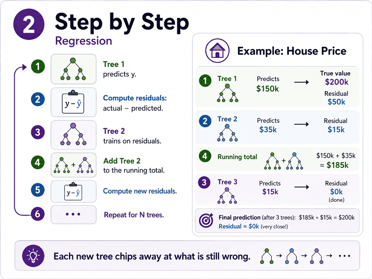
2. Step by Step:

For regression:

Tree 1. Predict y. It will be roughly right but make errors.
Compute residuals: actual − predicted.
Tree 2. Train it to predict those residuals.
Add Tree 2's prediction to Tree 1's. The combined model is now better.
Compute new residuals. Train Tree 3 on those. Add to the running total.
Repeat for N trees.

Each new tree chips away at what is still wrong. The model improves step by step.

A tiny concrete example. Say we are predicting house prices, true value = $200k.

Tree 1 predicts $150k → residual is $50k.
Tree 2 trains to predict that $50k residual. It guesses $35k.
Running total prediction is now $150k + $35k = $185k. Closer.
Tree 3 trains on the remaining $15k residual.

Three trees, getting steadily closer to $200k. That is the entire boosting loop. For classification, the same idea but using probabilistic residuals instead of raw errors.

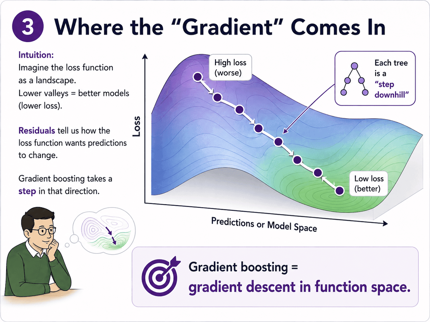
3. Where the "Gradient" Comes In:

The name gradient boosting hints at gradient descent (Day 7: Gradient Descent — How Models Actually Learn). Residuals are basically saying "here is how the loss function would want us to change the prediction." Gradient boosting builds a tree that takes a step in that direction. So it is gradient descent, but in function space instead of parameer space. Each tree is a "step downhill" on the loss surface.

We do not need this depth for interviews. But the name now makes sense.

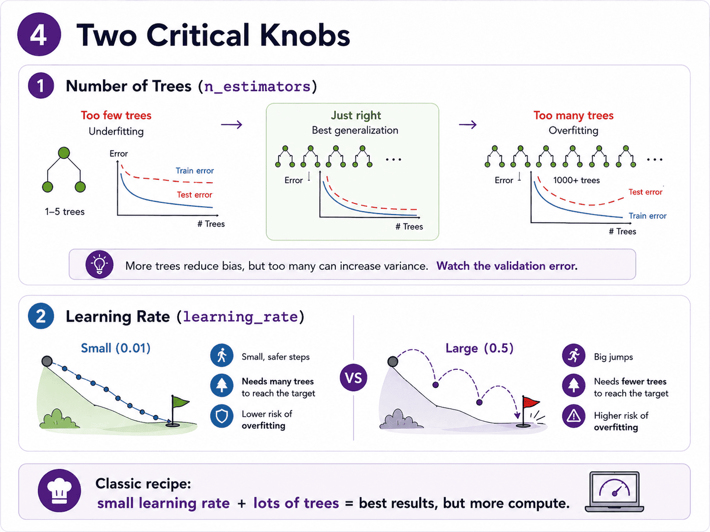
4. Two Critical Knobs:

Number of trees (n_estimators). More trees means more chances to fix errors, but also more chances to overfit. Unlike Random Forest, gradient boosting can overfit by adding too many trees. We use early stopping or cross-validation to find the sweet spot.

Learning rate (learning_rate). Each tree's contribution is shrunk by the learning rate (for example, 0.1).

Small learning rate (0.01): each tree makes a small fix. We need many trees, but the model generalises better.
Big learning rate (0.5): each tree makes a big fix. Few trees needed, but easy to overfit.

The classic recipe is small learning rate plus lots of trees gives the best results, at the cost of more compute. There is a beautiful interplay here. Lower learning rate but more trees usually trades compute for accuracy. We tune both together.

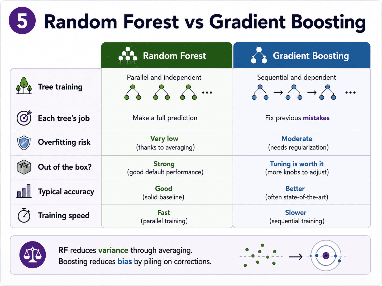
5. Random Forest vs Gradient Boosting:

Aspect	Random Forest	Gradient Boosting
Tree training	Parallel, independent	Sequential, dependent
Each tree's job	Full prediction	Fix previous mistakes
Overfitting risk	Very low	Moderate (needs care)
Out of the box?	Yes	Tunes are worth it
Typical accuracy	Good	Better
Training speed	Fast (parallel)	Slower (sequential)

Both are tree ensembles. Their philosophies are opposite. RF reduces variance through averaging. Boosting reduces bias by piling on corrections.

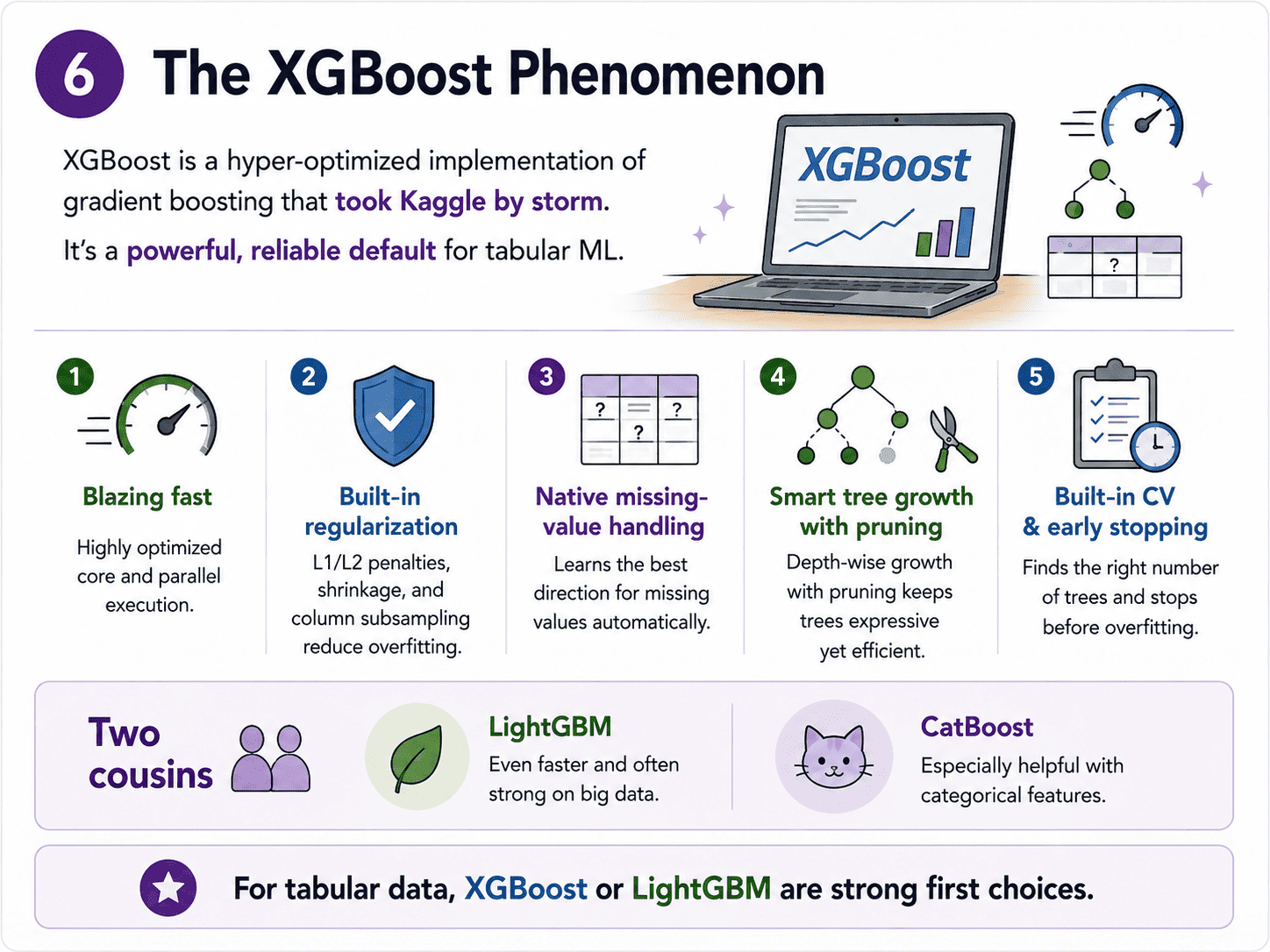
6. The XGBoost Phenomenon:

XGBoost (eXtreme Gradient Boosting) is a hyper-optimised implementation. It dominated Kaggle for years for good reasons.

Massive speed (parallel feature processing, GPU support).
Built-in regularisation (L1/L2 on leaf weights).
Native handling of missing values.
Smart tree growth (level-wise, with pruning).
Built-in cross-validation and early stopping.

Two cousins worth knowing.

LightGBM: even faster, leaf-wise tree growth. Often beats XGBoost on big data.
CatBoost: native support for categorical features. Less fiddling.

If an interviewer asks "what would you reach for on a tabular dataset?", the right answer is XGBoost or LightGBM.

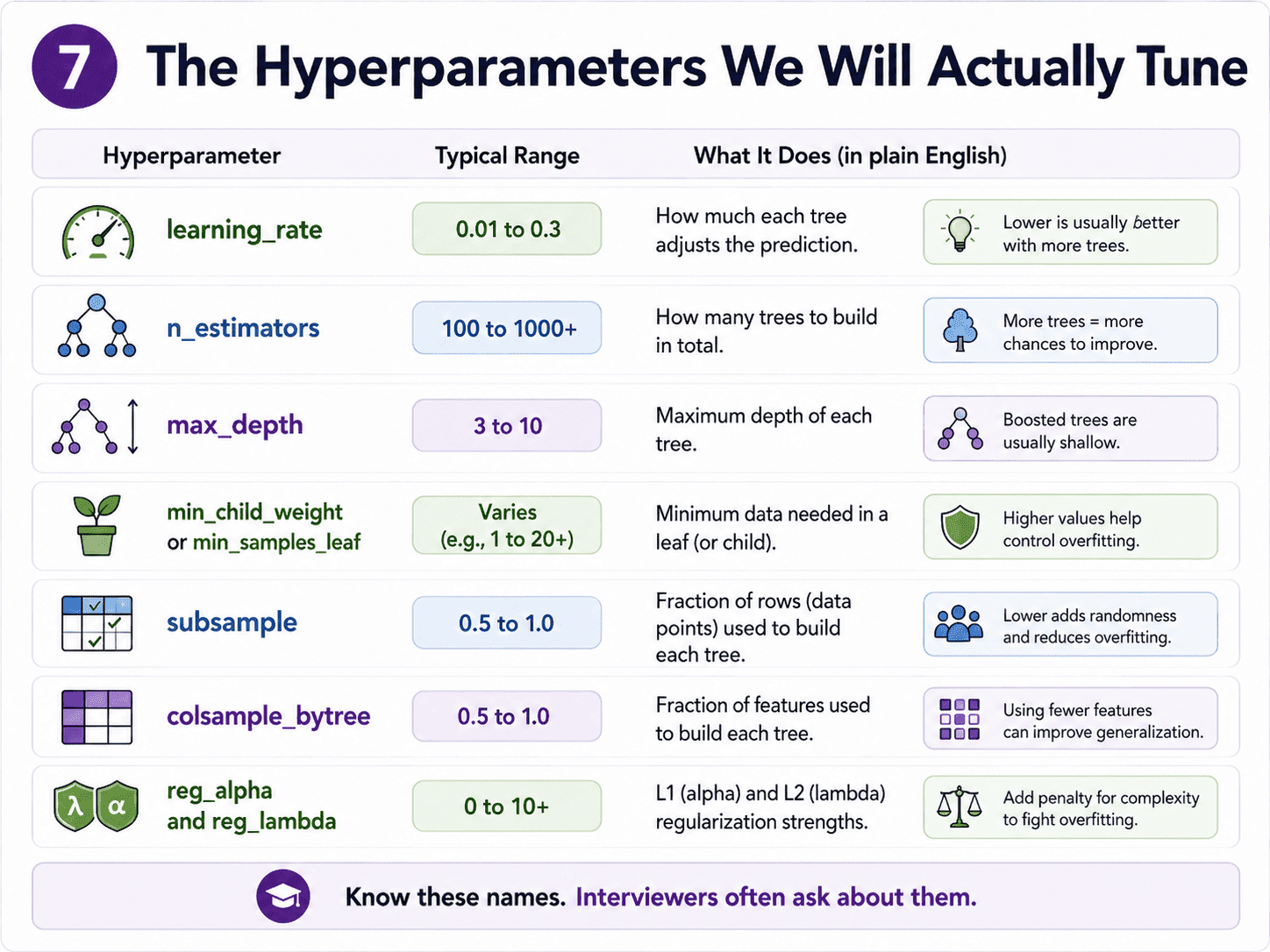
7. The Hyperparameters We Will Actually Tune:

The shortlist worth memorising.

learning_rate: 0.01 to 0.3 (lower is usually better with more trees).
n_estimators: 100 to 1000+.
max_depth: 3 to 10 (boosted trees are usually shallow).
min_child_weight / min_samples_leaf: controls overfitting.
subsample: fraction of rows per tree (bagging-style randomness).
colsample_bytree: fraction of features per tree.
reg_alpha / reg_lambda: L1 and L2 regularisation.

Memorise the names. Interviewers like to check that we can talk this fluently.

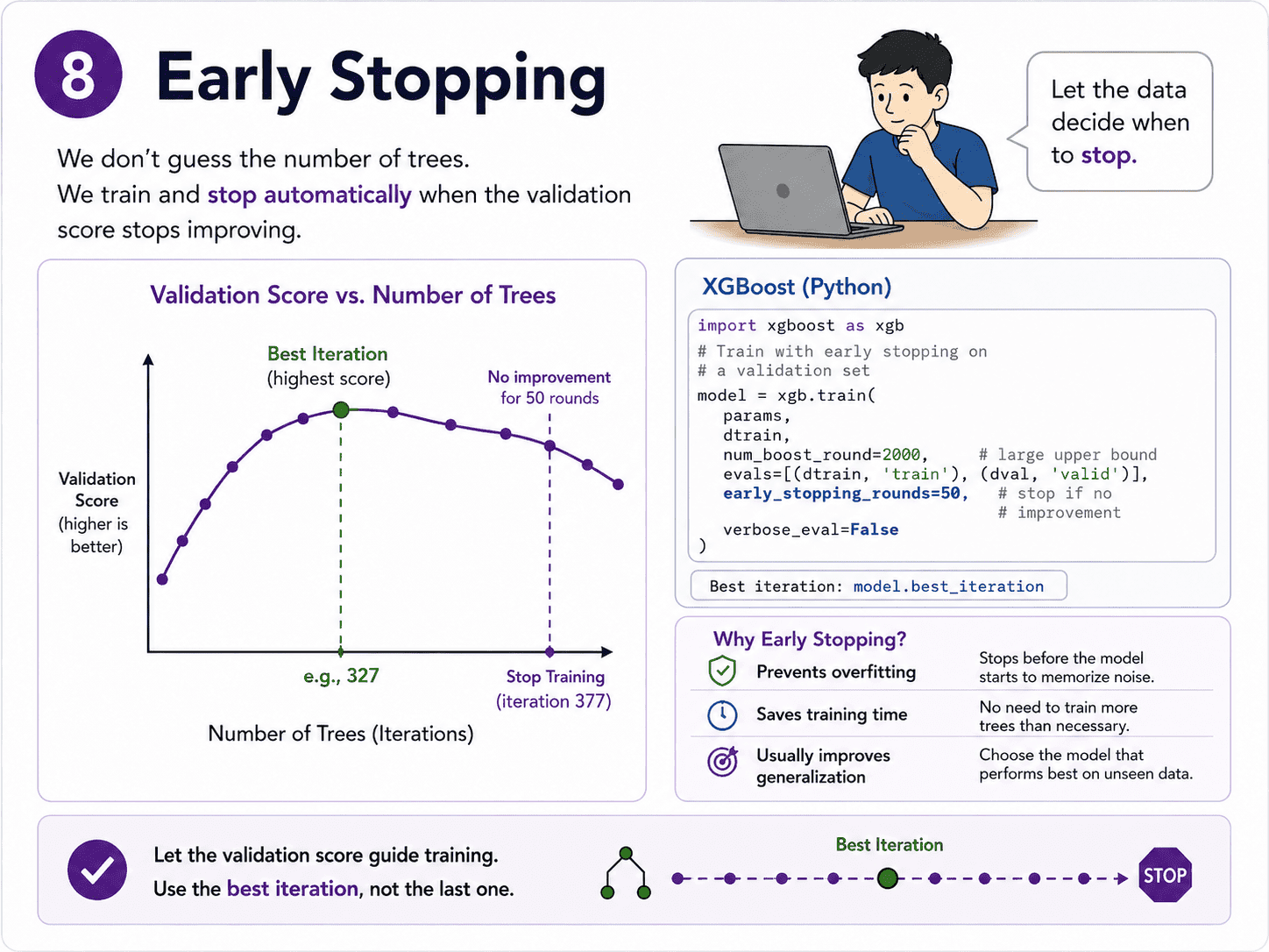
8. Early Stopping:

We do not guess n_estimators. We train with a validation set and stop when its score stops improving.

import xgboost as xgb

model = xgb.XGBClassifier(
    learning_rate=0.05,
    n_estimators=5000,
    max_depth=6,
    eval_metric='auc',
    early_stopping_rounds=50
)

model.fit(
    X_train, y_train,
    eval_set=[(X_val, y_val)],
    verbose=False
)

print("Best iteration:", model.best_iteration)

If the validation score does not improve for 50 rounds, training stops. We get the optimal model for free.

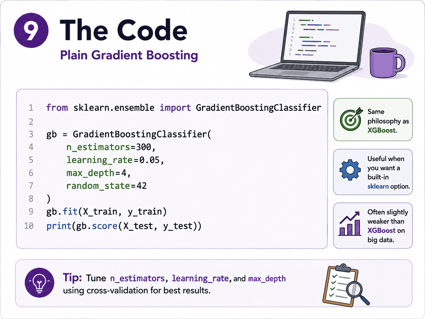
9. The Code (Plain Gradient Boosting):

If we do not want to install XGBoost, sklearn has its own version.

from sklearn.ensemble import GradientBoostingClassifier

gb = GradientBoostingClassifier(
    n_estimators=300,
    learning_rate=0.05,
    max_depth=4,
    random_state=42
)
gb.fit(X_train, y_train)
print(gb.score(X_test, y_test))

It is a few percentage points worse than XGBoost on big data, but identical in philosophy.

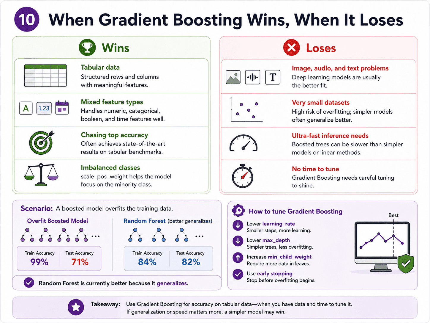
10. When Gradient Boosting Wins, When It Loses:

It wins on tabular data competitions and in production. On mixed feature types. When we are chasing every last percentage point. And on imbalanced classes (using scale_pos_weight in XGBoost).

It loses on image, audio, or text (deep learning destroys it). On tiny datasets (Random Forest is more stable). When inference must be ultra-fast (boosted trees are denser than RF). And when we do not have time to tune, since RF has fewer knobs.

A small thought to sit with.

Suppose our boosted model has 99% train accuracy and 71% test accuracy. We ship the same dataset to a Random Forest and get 84% train / 82% test. Which is "better," and what tuning would we try on the boosted model?

The Random Forest is currently better because it generalises. The boosted model is overfitting hard.

We would try lowering the learning rate (0.05 → 0.01), lowering max_depth (8 → 4), increasing min_child_weight, and using early stopping with a validation set.

Boosted models reach higher peaks than Random Forest, but they need careful tuning to get there. We should never compare untuned to untuned.

11. A Few Common Confusions Cleared:

What is "gradient" boosting vs "regular" boosting? Earlier boosting (AdaBoost) re-weighted misclassified examples each round. Gradient boosting generalises this. Each new tree fits the negative gradient of the loss function. Same idea, more general math, better performance.
Why are boosted trees usually shallow (depth 3 to 6)? Because the boosting framework adds many trees. Each tree only needs to capture a small piece of the pattern. Deep trees in this setting overfit fast.
Does it need scaling? No. Tree-based.
Why does XGBoost beat plain gradient boosting? Speed (parallelism, optimised C++), better regularisation, native missing-value handling, smarter tree-building. The algorithm idea is the same; the engineering is far better.
Common interview question: "Bagging vs Boosting?" Bagging = parallel models on different data, averaged to reduce variance (RF). Boosting = sequential models, each fixing the previous's mistakes, to reduce bias (XGBoost). Memorise that one line.

12. If This Came In An Interview:

A few questions to be ready for, with one-line answers.

What is gradient boosting? Training trees sequentially, where each new tree fits the residuals (mistakes) of the trees built so far.
Bagging vs Boosting? Bagging: parallel models on different random data, averaged to reduce variance (Random Forest). Boosting: sequential models, each fixing the previous's mistakes, to reduce bias (XGBoost).
What does the learning rate do in boosting? It shrinks each tree's contribution. Lower learning rate means smaller, safer steps. Small learning rate plus many trees usually gives the best results.
Why does XGBoost beat plain gradient boosting? Better engineering: parallelism, optimised C++ code, built-in regularisation, native missing-value handling, smarter tree-building. The algorithm idea is the same.
What is early stopping? Halting training when the validation score stops improving for N rounds. Avoids guessing the right number of trees.
How do you handle class imbalance in XGBoost? The scale_pos_weight parameter. Set it to the ratio of negatives to positives.
Why are boosted trees usually shallow? Because we add many trees. Each tree only needs to capture a small piece of the pattern. Deep trees overfit fast in this setting.

13. Summing It Up:

If we remember one thing from today, it is this: each new tree fixes the previous tree's mistakes. Small learning rate plus many trees usually wins. XGBoost and LightGBM are the workhorses of competitive tabular ML, and a strong default in industry. Use early stopping to find the right number of trees automatically.

Coming Up on Day 17: Support Vector Machines — Drawing the Widest Lane

We have now covered KNN, Naive Bayes, Decision Trees, Random Forest, and XGBoost. Tomorrow we wrap up supervised learning with a classic that uses pure geometry to draw the boundary between classes: Support Vector Machines. SVMs were favourites in the 2000s, are still useful today, and they give the cleanest illustration of the famous kernel trick.

That's all for today. Let's meet up again tomorrow with Day 17.

Thanks for reading.

Cheers!