Day 13: Naive Bayes — Bayes' Rule Goes to Work

Yesterday's KNN looked at neighbours. Today's algorithm takes a completely different route: pure probability.

Naive Bayes is the algorithm that quietly powers most of the world's spam filters, and it is one of the easiest probabilistic models to wrap our heads around.

This blog post is a daily learning summary of my ML self-study.

Terms Used Today

Conditional probability: P(A | B), the chance of A given that B is true.

Prior probability: Our belief in a class before seeing any features (often the base rate in training data).

Bayes' theorem: A way to flip conditionals. P(A | B) = P(B | A) × P(A) / P(B).

The "naive" assumption: Treat features as independent given the class.

Laplace smoothing: Add a small count to every feature so unseen words do not zero out the probability.

Generative model: Models how the data was generated and uses Bayes to flip it (contrasts with discriminative models like Logistic Regression).

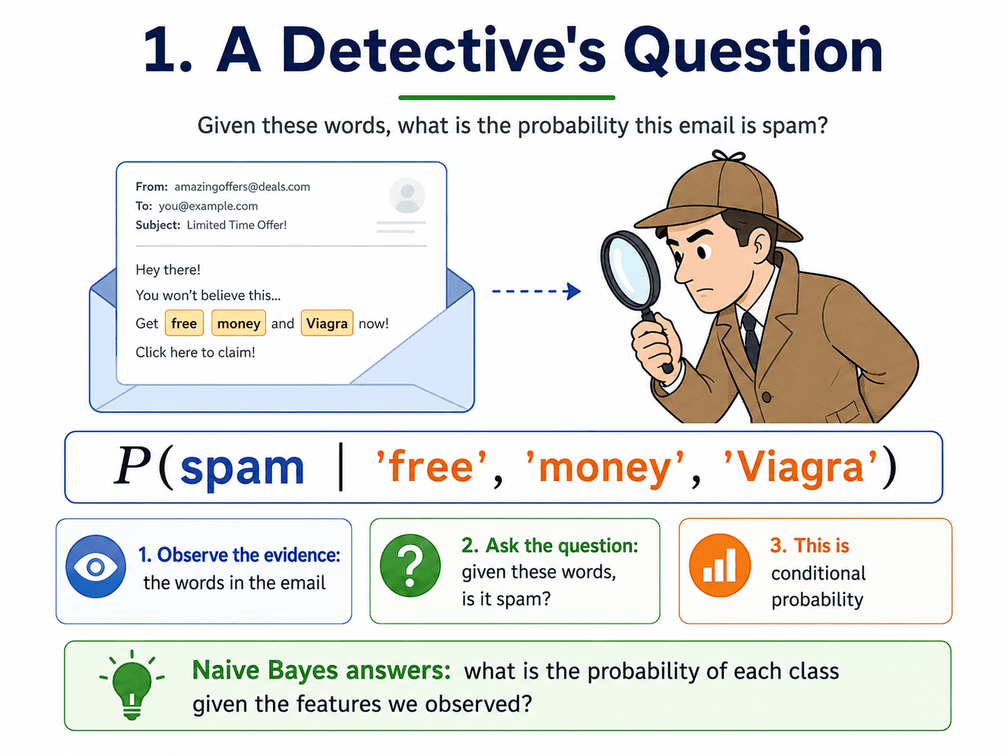
1. A Detective's Question:

Imagine we are detectives. We see an email containing the words "free," "money," and "Viagra." We ask the question: "Given these words, what are the chances this is spam?"

In symbols, this is:

P(spam | "free", "money", "Viagra")

That is a conditional probability, the probability of one thing given another. This is exactly what Naive Bayes computes.

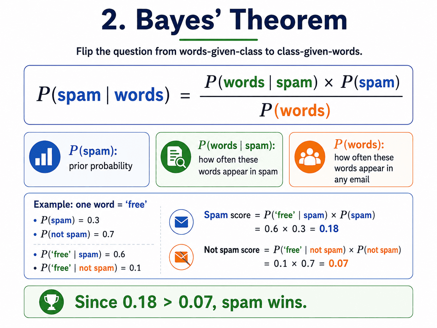
2. Bayes' Theorem:

The math looks scary, but it is friendlier than it looks.

P(A | B) = [ P(B | A) × P(A) ] / P(B)

In plain English, for our spam problem:

P(spam | words) = [ P(words | spam) × P(spam) ] / P(words)

Three pieces.

P(spam): how often is any email spam? (the prior).
P(words | spam): how often do these words appear in spam emails?
P(words): how often these words appear in any email (we mostly ignore this for prediction).

We combine them and we get the probability we want. That is Bayes' theorem.

A tiny number example. Say 30% of emails are spam (P(spam) = 0.3, P(not-spam) = 0.7). The word "free" appears in 60% of spam emails and 10% of legitimate emails. For a new email containing "free":

Spam side: P("free" | spam) × P(spam) = 0.6 × 0.3 = 0.18
Not-spam side: P("free" | not-spam) × P(not-spam) = 0.10 × 0.7 = 0.07

Spam wins, with a score about 2.6× higher than not-spam. To turn these into actual probabilities, we divide each by their sum: P(spam | "free") ≈ 0.18 / 0.25 = 72%. For picking the winner, though, the raw scores are enough.

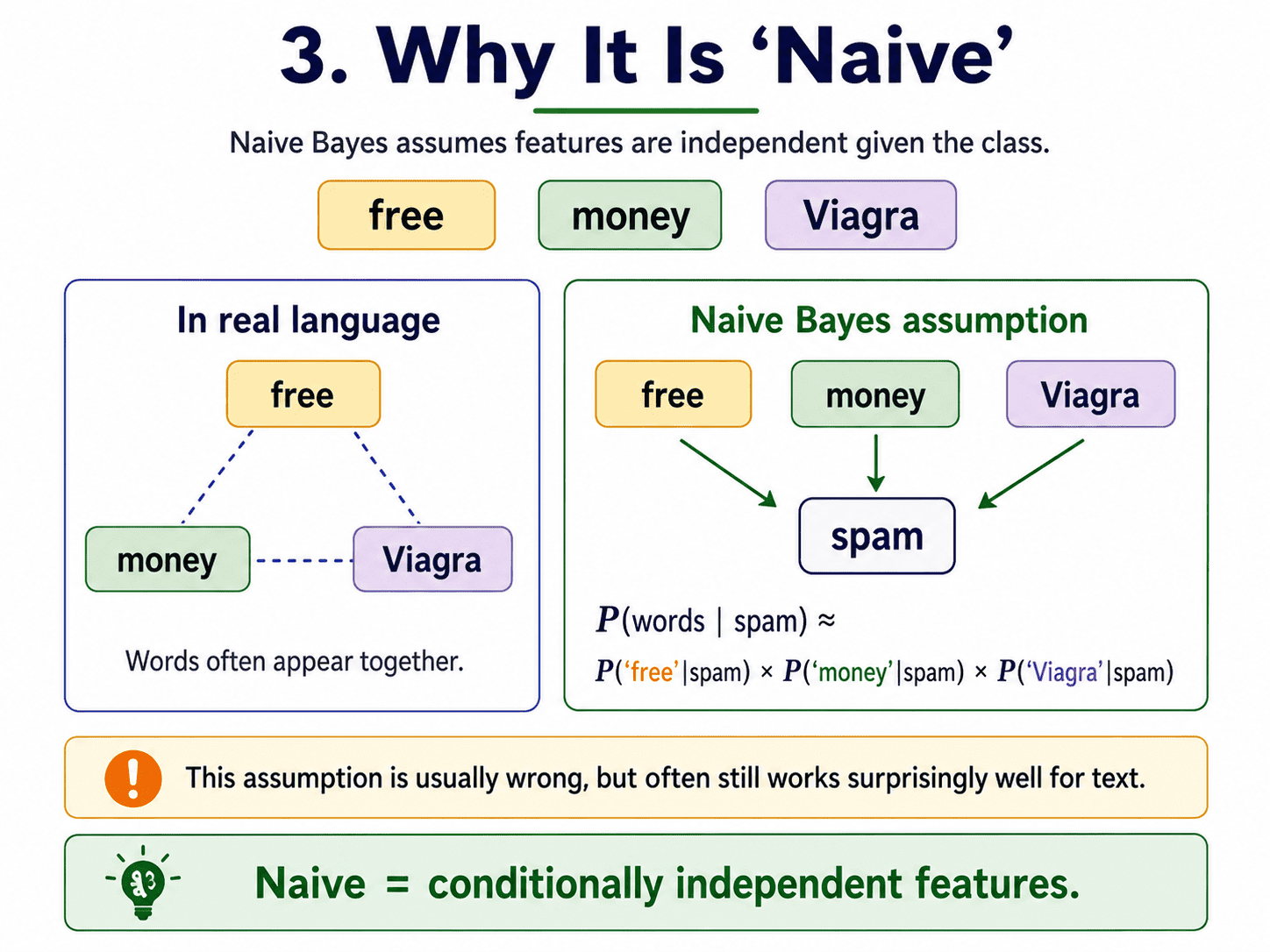
3. Why "Naive"?

The "words" part is multiple features at once: "free" AND "money" AND "Viagra." Computing P(all those words together | spam) is hard, because words in real language are correlated.

So Naive Bayes makes a wildly simplifying assumption: assume every feature is independent of every other.

P(words | spam) ≈ P("free" | spam) × P("money" | spam) × P("Viagra" | spam)

This is laughably wrong in real language. "Free" in an email is way more likely to appear near "money" than near "Tuesday." And yet, Naive Bayes works shockingly well, especially for text. Hence the name. It is naively assuming independence, but the trick pans out in practice.

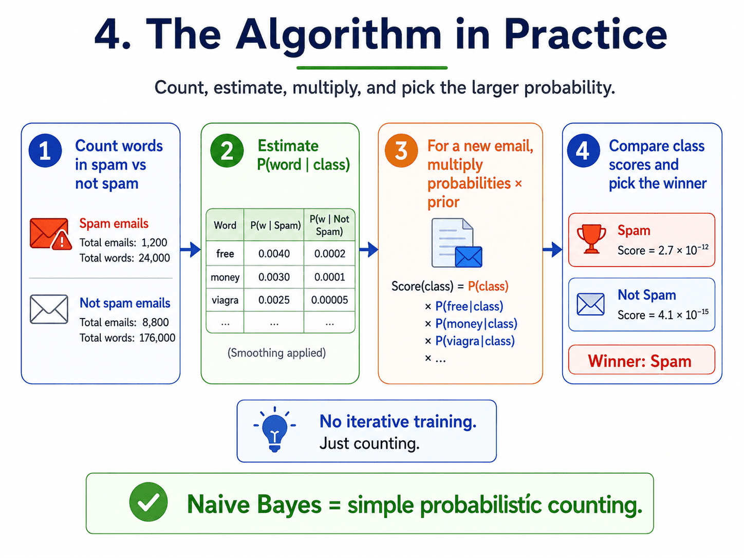
4. The Algorithm in Practice:

Count how often each word appears in spam emails vs not-spam emails.
From those counts, estimate P(word | spam) and P(word | not-spam).
For a new email, multiply the probabilities together, weighted by the prior.
Whichever class has the higher probability wins.

That is the entire algorithm. No optimisation, no iterations. Just counting.

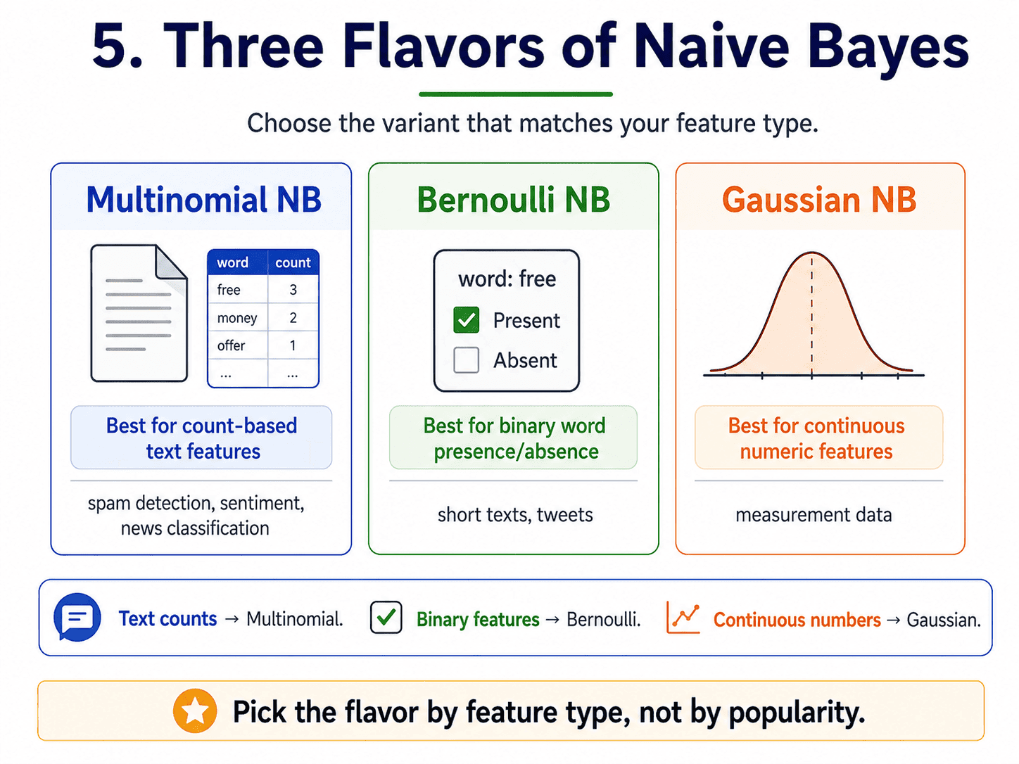
5. Three Flavors:

sklearn ships three versions.

Multinomial NB. For count-based features. The classic for text classification, where features are word counts in documents.

from sklearn.naive_bayes import MultinomialNB
model = MultinomialNB()

Bernoulli NB. For binary features: "did the word appear or not?" Useful for short texts like tweets.

from sklearn.naive_bayes import BernoulliNB

Gaussian NB. For continuous numeric features. Assumes each feature is normally distributed within each class.

from sklearn.naive_bayes import GaussianNB

We pick the flavor by feature type. Text? Multinomial. Yes/no features? Bernoulli. Numbers? Gaussian.

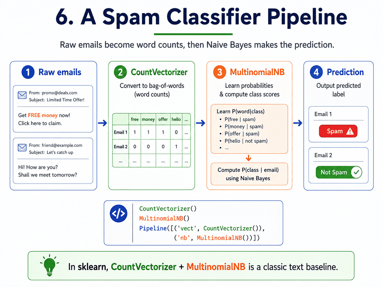
6. A Spam Classifier:

from sklearn.feature_extraction.text import CountVectorizer
from sklearn.naive_bayes import MultinomialNB
from sklearn.pipeline import Pipeline

pipe = Pipeline([
    ('vectorizer', CountVectorizer()),
    ('nb', MultinomialNB())
])

pipe.fit(emails_train, labels_train)
pipe.score(emails_test, labels_test)

CountVectorizer turns raw text into word counts. MultinomialNB learns the probabilities. Two lines of training, and we have a working spam filter.

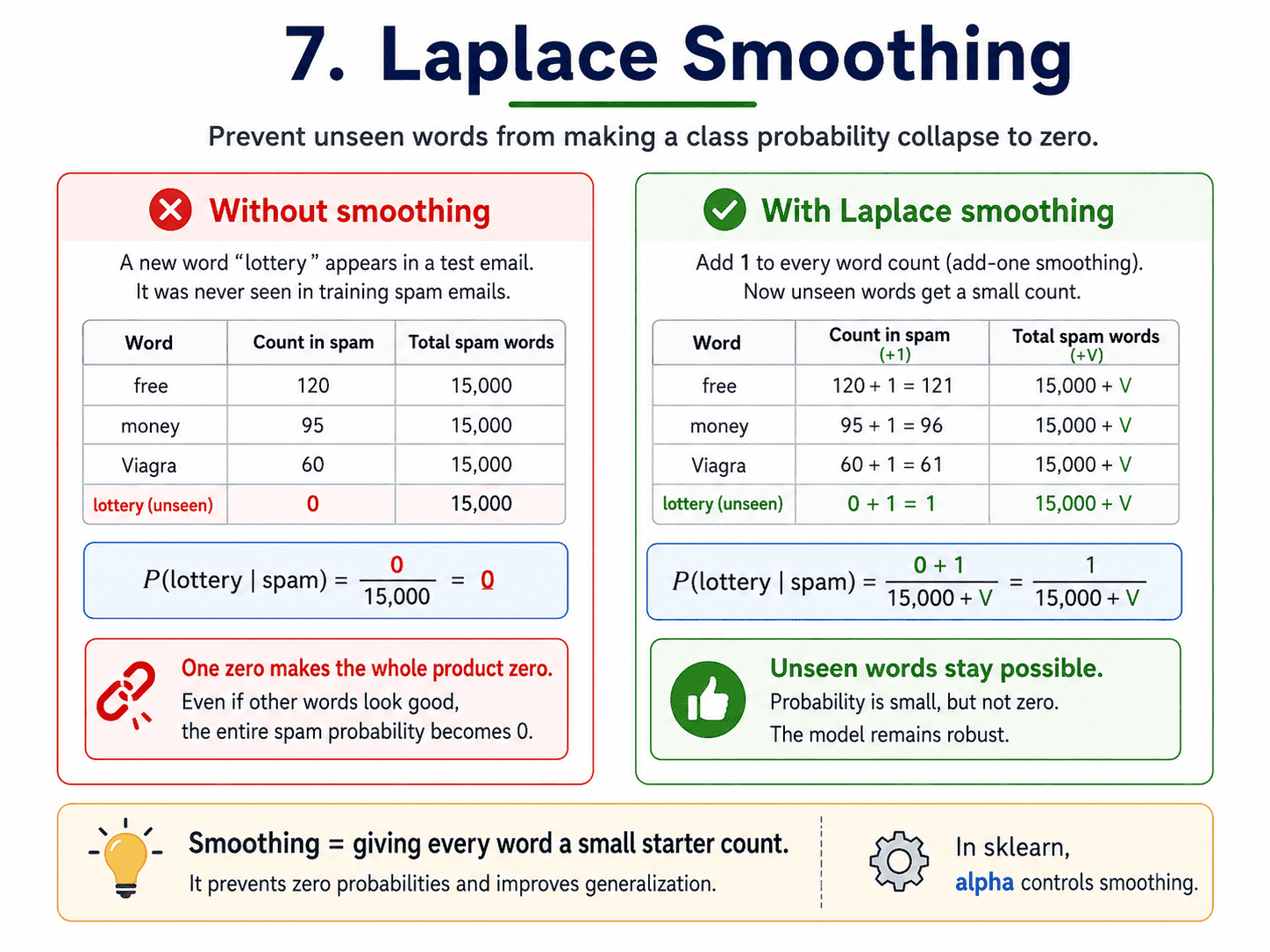
7. Laplace Smoothing:

What if a test email contains a word the model has never seen in spam? Then P(word | spam) = 0. Multiply anything by zero and the whole probability collapses to zero. To prevent this, we add a tiny pseudocount (usually 1) to every word count. This is called Laplace smoothing.

sklearn does this automatically via the alpha parameter (default 1.0). We rarely need to touch it.

8. Why It Wins on Text:

Three reasons Naive Bayes is the eternal text-classification favourite.

Fast. Training is just counting. Prediction is just multiplication.
Scales. Millions of documents, no problem.
Robust. Surprisingly resistant to irrelevant words, since each feature contributes independently.

Modern transformers crush Naive Bayes on hard NLP tasks. But for "is this email spam?" or "is this review positive or negative?", Naive Bayes is still a serious baseline.

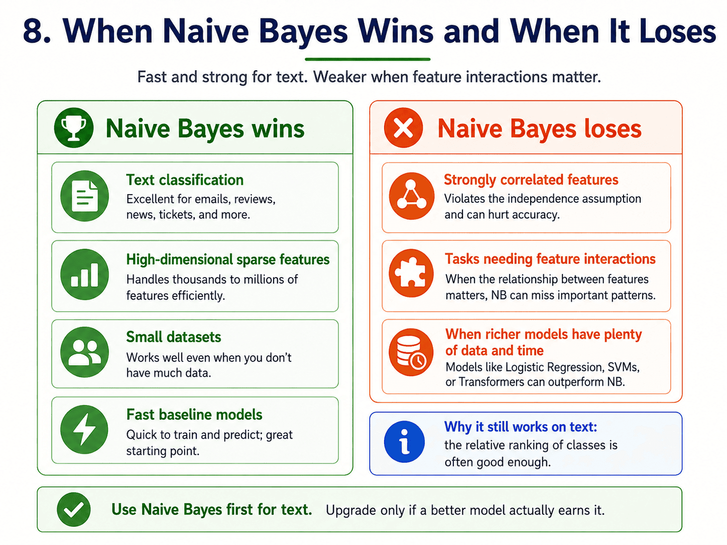
9. When Naive Bayes Wins, When It Loses:

It wins on text classification (spam, sentiment, news categorisation), on small datasets where it still gives sensible results, on high-dimensional features (thousands of words, because the independence assumption hurts less as dimensions grow), and when we want a fast, sensible baseline before reaching for anything heavy.

It loses when features are strongly correlated (like height and weight), when the task requires modelling feature interactions, or when we have lots of data and lots of time, in which case a richer model usually wins.

A small thought to sit with. Imagine a Gaussian Naive Bayes classifier for diagnosing a disease, using two features: blood pressure and weight. Body weight and blood pressure are strongly correlated in real patients.

Does this break Naive Bayes?

Should we abandon it? Strictly speaking, yes, the independence assumption is violated. But in practice, Naive Bayes is famously robust to this kind of violation.

It often still works fine, because the ranking of class probabilities tends to be right even when the absolute values are off. We test it as a baseline first, and we move on only if it actually underperforms.

10. A Few Common Confusions Cleared:

What is a "prior probability"? Our belief about a class before seeing any features. Often, it is just the proportion of each class in the training data. For example, P(spam) = 0.3 if 30% of training emails are spam.
Is Naive Bayes a generative or discriminative model? Generative. It models how the data was generated (P(words | spam)) and uses Bayes to flip the question. Logistic Regression, by contrast, is discriminative: it directly models P(spam | words). This is a frequently asked interview distinction.
Why does Naive Bayes work on text despite the wrong assumption? Because in high-dimensional text, the cumulative product of many features overwhelms the dependence violations. The model only needs the relative probabilities to be roughly right, not the absolute values.
Does Naive Bayes need scaling? No. It works with counts and probabilities, not distances or gradients.
Common interview question: "What does naive mean in Naive Bayes?" It naively assumes that all features are conditionally independent given the class, even when they are not. Despite the wrong assumption, it works well in practice, especially on text.

11. If This Came In An Interview:

A few questions to be ready for, with one-line answers.

What does "naive" mean in Naive Bayes? It naively assumes that all features are conditionally independent given the class. Usually wrong, but the algorithm still works well in practice.
Is Naive Bayes a generative or discriminative model? Generative. It models how the data was generated (P(features | class)) and uses Bayes' theorem to flip the question.
Why does it work well on text despite the wrong assumption? In high-dimensional text, the cumulative product of many features overwhelms the dependence violations. The ranking of class probabilities is usually right.
What is Laplace smoothing? Adding a small pseudocount (usually 1) to every word count so that an unseen word does not drive a class probability to zero.
Multinomial vs Bernoulli vs Gaussian NB, when to use each? Multinomial for word counts (text), Bernoulli for binary presence/absence features, Gaussian for continuous numeric features.
Does Naive Bayes need feature scaling? No, because it works with counts and probabilities, not distances or gradients.

12. Summing It Up:

If we remember one thing from today, it is this: Naive Bayes counts how often words appear in each class, multiplies the probabilities, and picks the highest one. No optimisation. Just counting. It naively assumes features are independent (usually wrong, rarely fatal), and it remains the go-to baseline for text classification.

Coming Up on Day 14: Decision Trees — Twenty Questions Automated

We have seen distance-based (KNN) and probability-based (Naive Bayes) classifiers. Tomorrow we meet the most interpretable classifier of all, the one we can literally draw on a whiteboard and follow with our finger: Decision Trees. Behind every Random Forest and XGBoost we will meet next week is one of these.

That's all for today. Let's meet up again tomorrow with Day 14.

Thanks for reading.

Cheers!