Day 12: K-Nearest Neighbors — Tell Me Who Your Friends Are

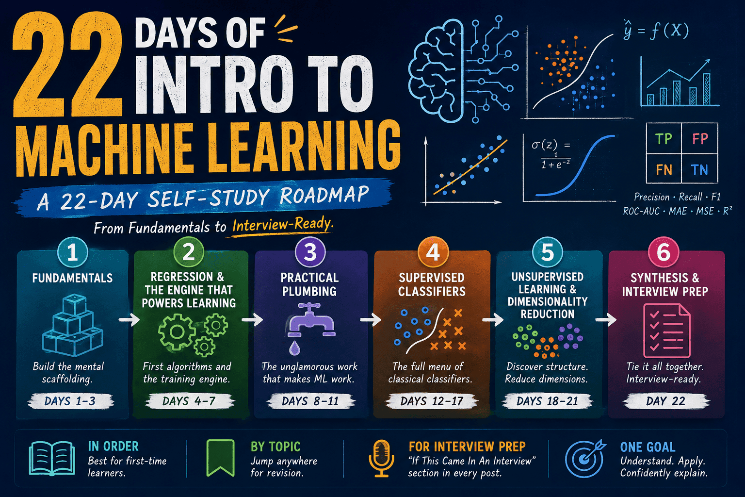
Eleven days of preparation and we are finally meeting our first classification algorithm beyond Logistic Regression. KNN (K-Nearest Neighbours) is the most beginner-friendly algorithm of all. It has no math to memorise, no training phase, and a one-line intuition we will never forget.

This blog post is a daily learning summary of my ML self-study.

Terms Used Today

KNN: Predict by looking at the K most similar training points and voting.

Lazy learning: No real training phase. All the work happens at prediction time.

Distance metric: How we measure "similar." Euclidean, Manhattan, cosine, etc.

K: The number of neighbours we consult. The only real hyperparameter.

Curse of dimensionality: In high-dimensional spaces, distances become meaningless. KNN suffers.

1. The One-Line Intuition:

"Tell me who your friends are, and I will tell you who you are."

If we want to know whether a new transaction is fraud, we look at the 5 most similar past transactions. If 4 of them were fraud, we predict fraud.

That is K-Nearest Neighbours in its entirety. No equations, no optimisation, no loss function. Just look at the neighbours.

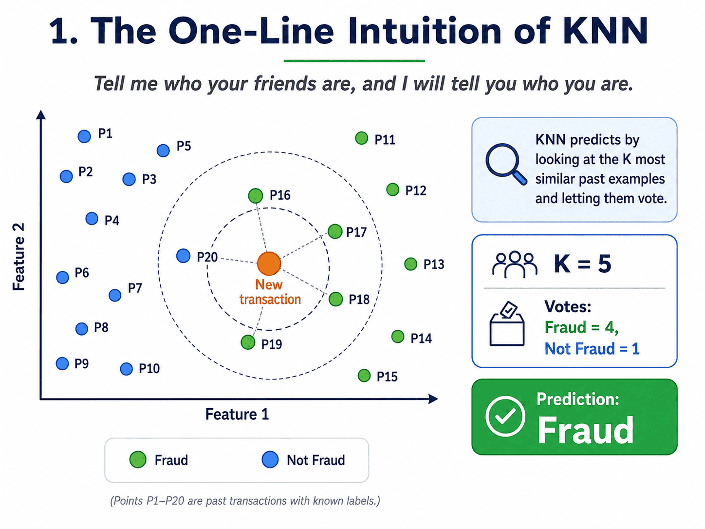
2. How It Works in 4 Steps:

For a new data point we want to classify:

Measure the distance from this point to every training point.
Pick the K nearest ones.
Look at their labels.
Vote: the most common label wins.

For regression, we replace "vote" with "average the K neighbours' values."

The whole algorithm fits in those four lines.

A tiny concrete example.

Say K = 3, and the three nearest neighbours of a new point have labels: fraud, fraud, not-fraud.

Vote count: 2 fraud, 1 not-fraud. Prediction: fraud. That is the whole decision.

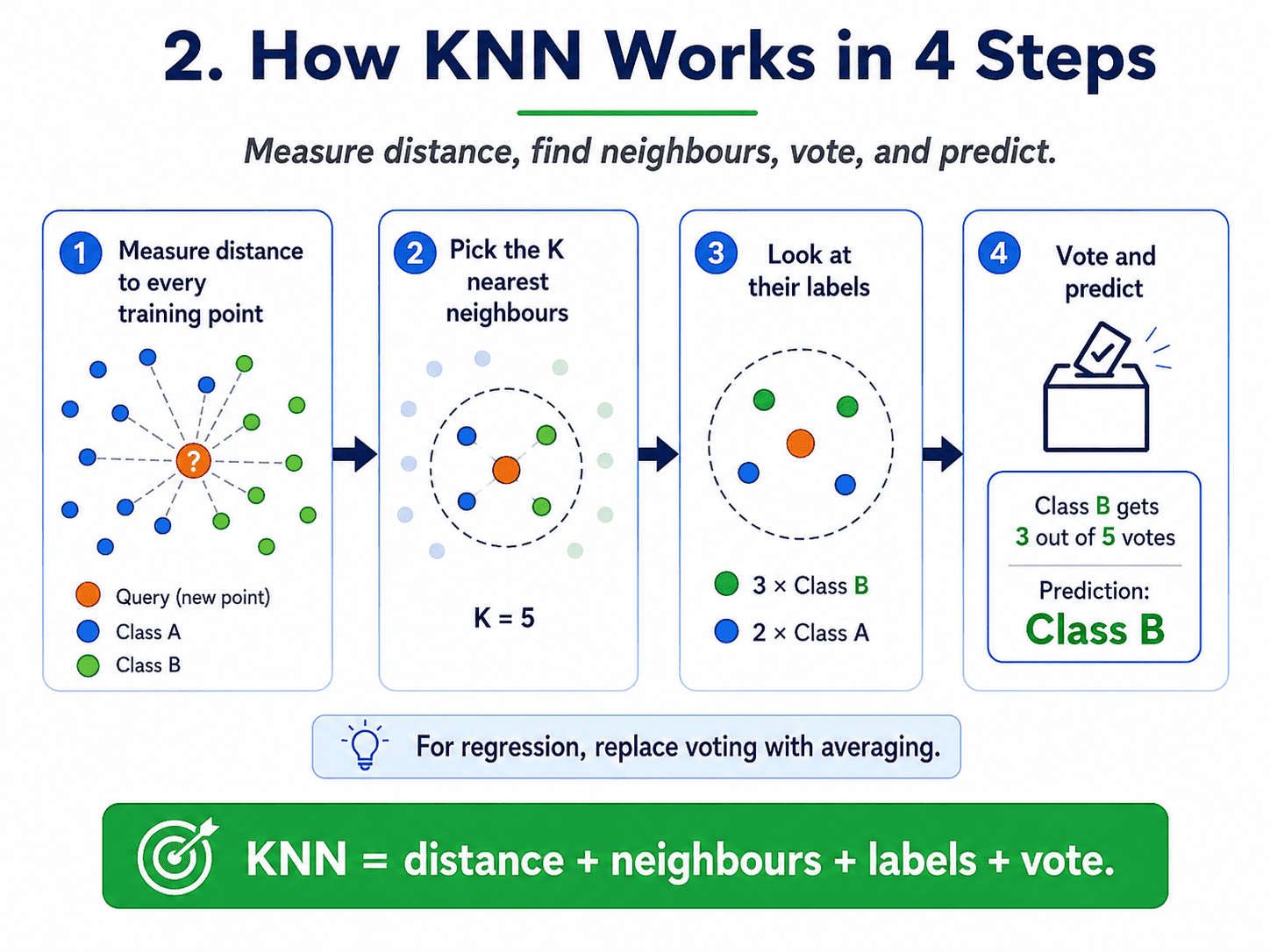
3. Why It Is Called "Lazy Learning":

Most algorithms train hard upfront and predict instantly. KNN flips this around.

Training: Literally just stores the dataset. Zero work.
Prediction: Computes distances to every training point. Lots of work.

KNN is lazy because it puts off all the thinking until we ask a question. This is its blessing (simplicity) and its curse (slow at prediction time on big data).

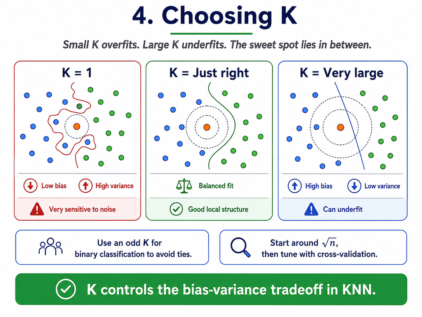
4. Choosing K:

The only real knob is how many neighbours to look at.

K = 1. Use only the closest neighbour. Super flexible. Overfits like crazy, because one noisy training point poisons the model in its local neighbourhood.
K very large. Averaging over the whole dataset. Underfits. Every prediction approaches the global majority class.
K just right. Smooth and accurate decisions.

If that sounds familiar, it should. It is the bias-variance seesaw from [[Day 3 Bias-Variance Tradeoff — Why Models Fail|Day 3]].

Small K = low bias, high variance.
Large K = high bias, low variance.

A typical starting point is K equal to the square root of the training-set size. We tune from there using cross-validation.

A small practical tip. Use an odd K for binary classification so votes do not tie.

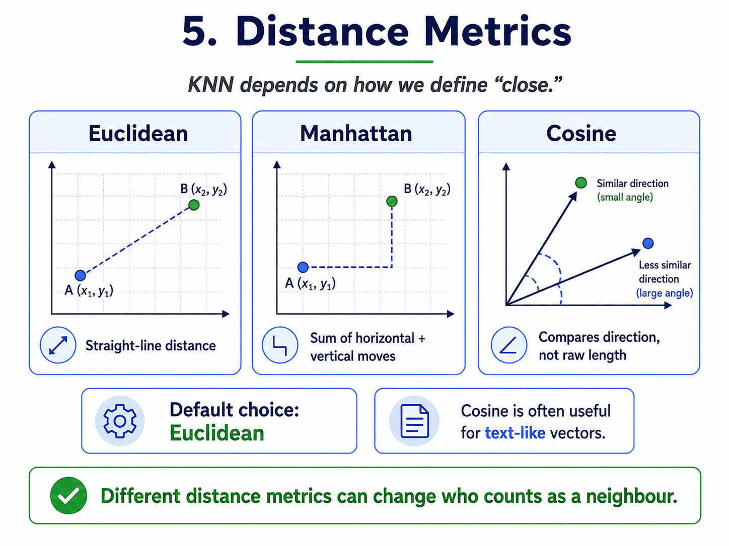
5. Distance Metrics:

KNN depends on a notion of "close." The default is Euclidean distance, the straight-line distance from school.

d = √((x₁ − x₂)² + (y₁ − y₂)² + ...)

Other options:

Manhattan distance: sum of absolute differences (also called "city block" distance).
Cosine distance: measures the angle between vectors. Useful for text.
Minkowski distance: a generalisation of Euclidean and Manhattan.

For most problems, Euclidean is fine.

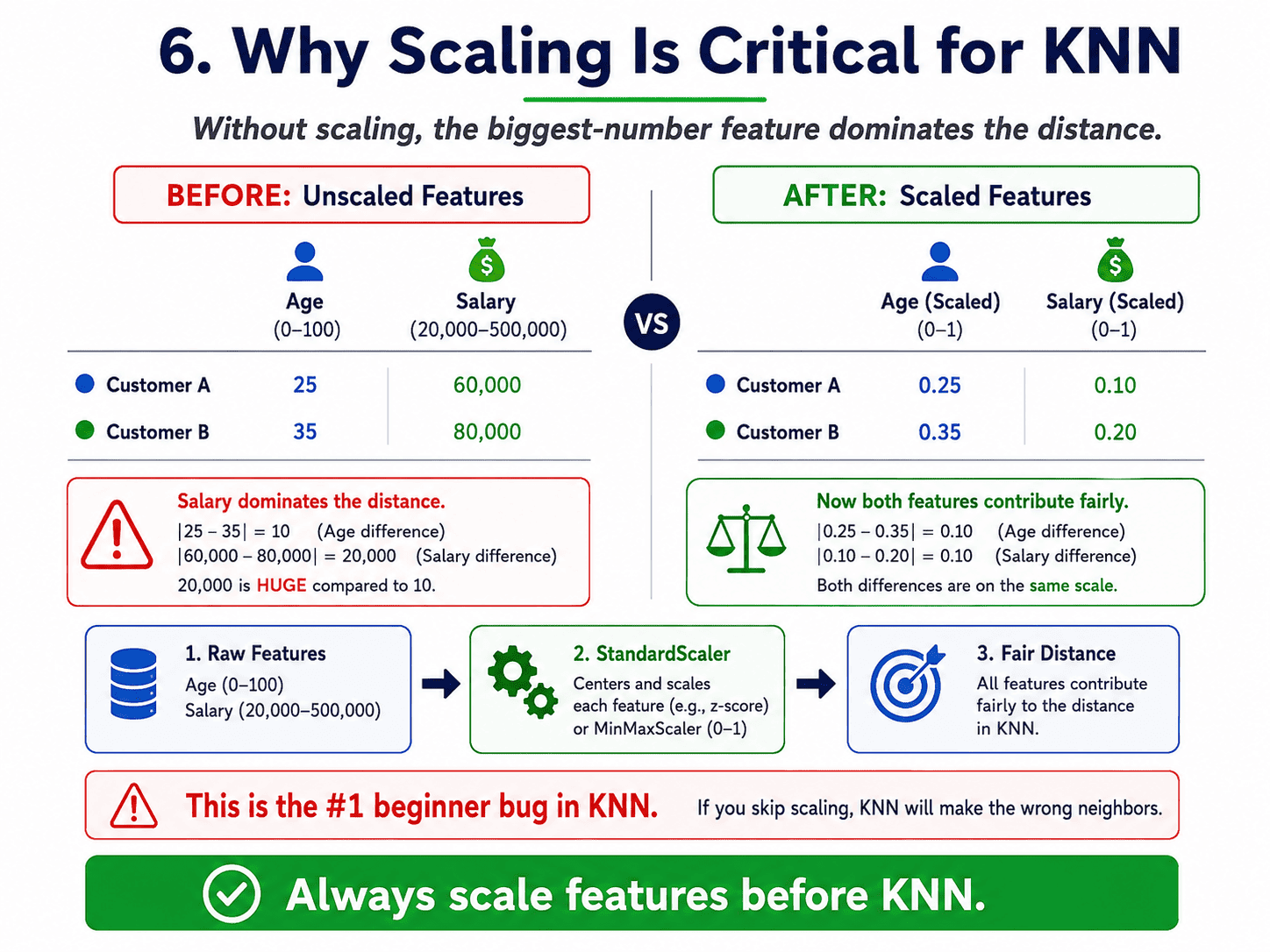
6. The Single Most Important Practical Rule:

We must scale our features before using KNN.

Why? Imagine two features:

Age: range 0 to 100.
Salary: range 20,000 to 500,000.

A 1-year age difference contributes about 1 to the distance.

A $1 salary difference also contributes 1. The salary feature completely dominates. Age becomes invisible.

We Standard-scale or Min-Max scale every feature so they contribute fairly. We covered this on Day 8: Feature Engineering & Preprocessing, but it is worth repeating, because forgetting this is the number one KNN beginner bug.

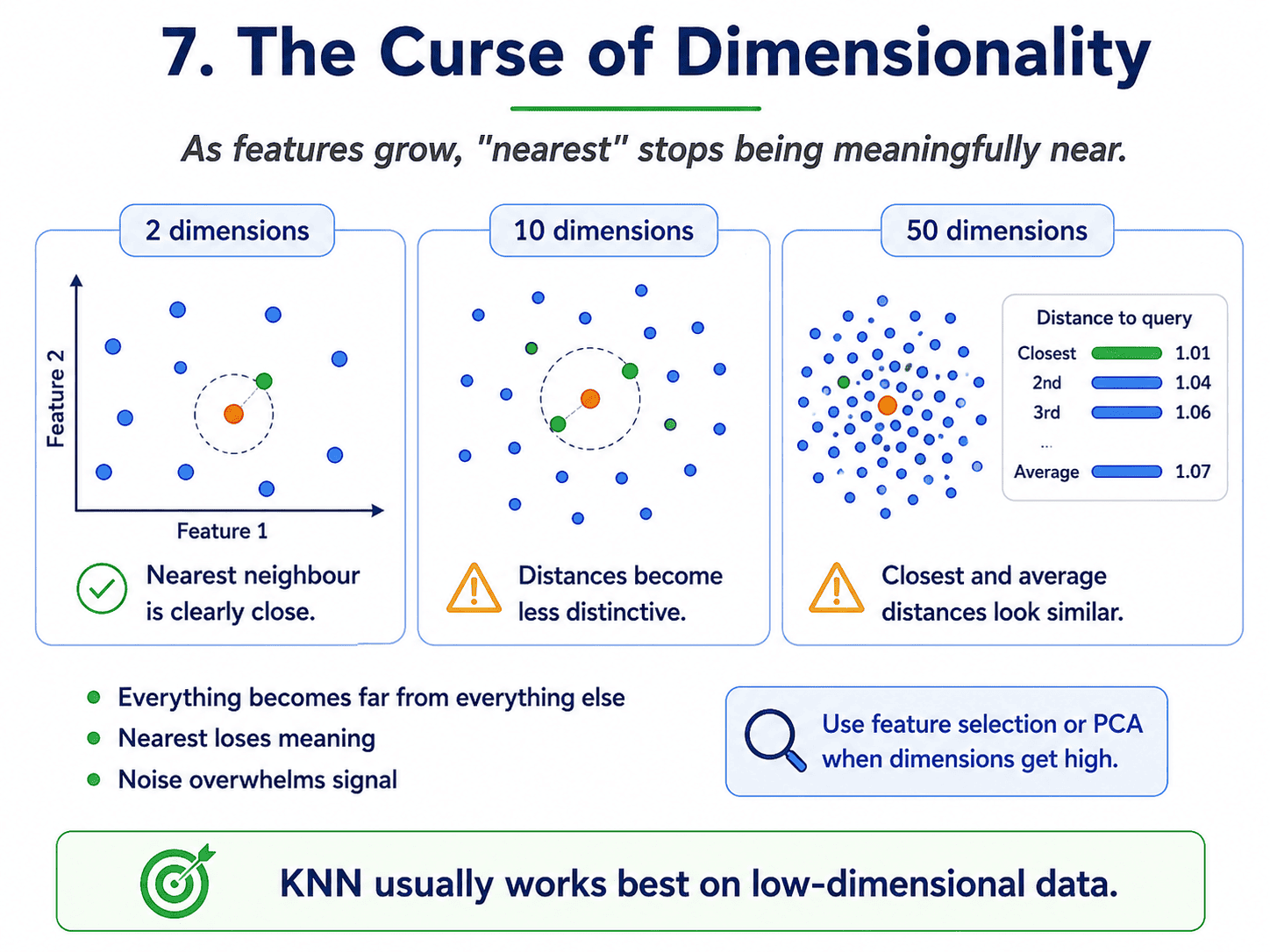
7. The Curse of Dimensionality:

KNN suffers as the number of features grows. In high dimensions:

Everything becomes far from everything else.
"Nearest" loses its meaning, because the closest neighbour is not meaningfully closer than the average.
Noise overwhelms signal.

Rule of thumb. KNN tends to struggle beyond about 20 features, unless we use feature selection or dimensionality reduction. Day 21: PCA — Shrinking Dimensions Without Losing Meaning (PCA) helps with this.

8. The Code:

from sklearn.preprocessing import StandardScaler
from sklearn.neighbors import KNeighborsClassifier
from sklearn.pipeline import Pipeline

pipe = Pipeline([
    ('scaler', StandardScaler()),   # critical
    ('knn', KNeighborsClassifier(n_neighbors=5))
])

pipe.fit(X_train, y_train)
pipe.score(X_test, y_test)

Two key arguments worth knowing:

n_neighbors: the K value.
weights='distance': closer neighbours vote more. Often gives a small boost.

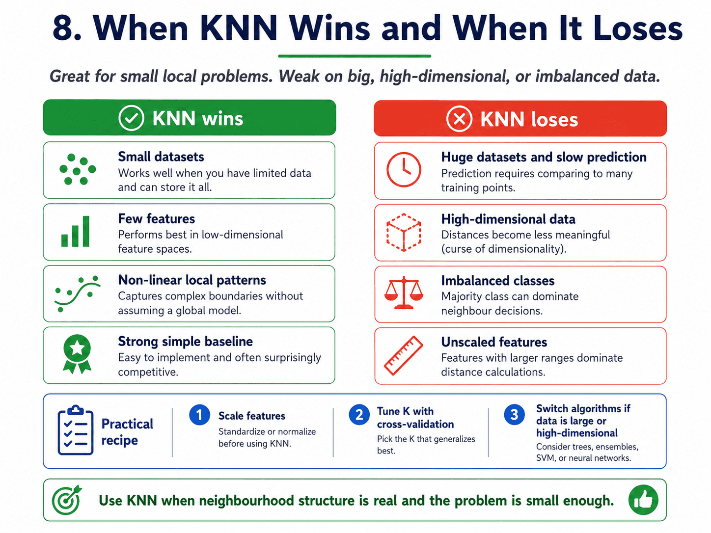
9. When KNN Wins, When It Loses:

It wins on small datasets where simplicity beats sophistication, when we have a few features with clear neighbourhood structure, when we want a strong baseline without thinking, and when decision boundaries are non-linear and local, because KNN naturally draws curvy boundaries.

It loses on huge datasets (every prediction touches every training point, which is slow), on high-dimensional data (curse of dimensionality), on imbalanced data (majority class dominates the neighbourhood), and when features are on different scales without scaling.

A small thought to sit with. Suppose we are using KNN to classify customer complaints into categories, and our feature set has 50 dimensions, including word frequencies.

KNN runs slowly and gives mediocre accuracy. What would we try first?

Two things. First, dimensionality reduction (PCA or feature selection) to bring the count down to a sane number. Second, switching algorithms. Naive Bayes Day 13: Naive Bayes — Bayes' Rule Goes to Work) or a tree-based model handles 50+ features much more gracefully than KNN.

The KNN paradigm is wrong for high-dimensional text. Knowing when not to use an algorithm is just as valuable as knowing how to use it.

10. A Few Common Confusions Cleared:

Is KNN supervised or unsupervised? Supervised. It uses labels to vote. (There is also a related unsupervised KNN used for finding similar items, but that is a different use.)
Why is it called lazy exactly? Because it does no training. All the work happens at prediction time. Contrast this with Logistic Regression, which trains hard but predicts in microseconds.
How big can my training data be before KNN gets slow? Naively, predictions are O(n) per query. With clever indexing (KDTree, BallTree), sklearn brings this down to roughly O(log n), but it is still much slower than Logistic Regression. Beyond around 100k rows, we should consider alternatives.
Does it work for regression? Yes, via KNeighborsRegressor. Replace voting with averaging the K neighbours' values.
Common interview question: "Why does KNN need scaling but Decision Trees do not?" KNN uses distances; Decision Trees use per-feature thresholds. Distances are scale-sensitive; thresholds are not.

11. If This Came In An Interview:

A few questions to be ready for, with one-line answers.

How does KNN make a prediction? It looks at the K most similar training points and takes the majority vote (classification) or the average (regression).
What is K and how do you choose it? The number of neighbours to consult. We choose it using cross-validation. Small K overfits, large K underfits.
Why does KNN need feature scaling? Because it uses distance. A feature on a larger scale dominates the distance calculation and drowns out the others.
Why is KNN called "lazy learning"? Because it does no real training. It just stores the data. All the work happens at prediction time.
What is the curse of dimensionality and why does it hurt KNN? In high dimensions, all distances become similar, so "nearest" loses meaning. KNN struggles past around 20 features.
When would you choose KNN over Logistic Regression? When the decision boundary is non-linear and local, the dataset is small, and we want a strong baseline without much thinking.

12. Summing It Up:

If we remember one thing from today, it is this: KNN has no training. It just remembers, measures distance, and votes. Choose K with cross-validation, always scale the features, and watch out for the curse of dimensionality.

Great for small problems, slow for big ones, and the cleanest illustration of the bias-variance seesaw in action.

Coming Up on Day 13: Naive Bayes — Bayes' Rule Goes to Work

KNN looked at neighbours. Tomorrow's classifier takes a wildly different route, using probability theory and a wonderfully simple assumption to crush a problem KNN cannot touch: text classification.

Welcome to Naive Bayes, the algorithm that quietly powers most "is this spam?" decisions on Earth.

That's all for today. Let's meet up again tomorrow with Day 13.

Thanks for reading.

Cheers!